
Shock Phase Space
This example demonstrates how to trace ions across a collisionless shock and analyze their phase space distribution, inspired by the demo from IRF-matlab. We utilize Liouville's theorem (phase space density conservation), backward/forward tracing, and Monte Carlo sampling to reconstruct the distribution function.
using TestParticle
import TestParticle as TP
using StaticArrays
using Random
using VelocityDistributionFunctions
using CairoMakie
using Meshes

seed = 42;
Shock model
The shock is prescribed analytically: a tanh ramp in density and magnetic field together with the electric field from the generalized Ohm's law. The subsections below fix one ingredient at a time.
Upstream plasma parameters
The upstream state is isothermal, T_ion = T_e = 20 eV. Together with the field below it fixes the whole shock: the MHD jump conditions then give the compression ratio n_down / n_up = 2 and the downstream bulk speed, so nothing in the setup is a free knob that was tuned to make the pictures look nicer.
const T_ion = 20.0  # ion temperature [eV]
const vth_ion = sqrt(2 * TP.qᵢ * T_ion / TP.mᵢ) # ion thermal speed [m/s]
const V_sw = -400.0e3; # solar wind bulk speed [m/s]
Shock structure parameters
const n_up = 3.0e6 # upstream number density [m⁻³]
const n_down = 6.0e6 # downstream number density [m⁻³]
# tanh profile from n_up (x → +∞) to n_down (x → −∞)
const n_jump = 0.5 * (n_down - n_up) # half density jump [m⁻³]
const n_avg = 0.5 * (n_down + n_up) # mean density [m⁻³]
const shock_width = 5.0e3; # shock ramp width [m]
# Amplitude of the electron pressure jump across the ramp. It enters the electric field
# only through the pressure-gradient part of Ohm's law, `-∇p_e/(n_e q)`, with
# `p_e = n k_B T_e` and constant `T_e`, so `Δp_e = k_B T_e · n_jump`. It is *not* the solar
# wind dynamic pressure `n_up m_i V_sw² = 0.80 nPa`, two orders of magnitude larger.
const Δp_e = TP.qᵢ * T_ion * n_jump; # electron pressure jump across the ramp [Pa]
Magnetic field parameters
const B_normal = 1.7e-9 # shock normal component of B [T]
const B_mag = 9.8e-9 # upstream magnetic field magnitude [T]
# The shock normal is x̂, so θ_Bn follows from the two field strengths above.
const θ_Bn = acosd(B_normal / B_mag) # shock normal angle [degree]
println("Shock normal angle θ_Bn = $(round(θ_Bn; digits = 1))°")
Shock normal angle θ_Bn = 80.0°Tangential field jump
The shock is oblique, θ_Bn ≈ 80°, so the tangential field jump follows from the oblique-shock jump conditions. In the plasma frame, which is the frame E is written in, the transverse momentum balance ρ U_n ∂ₓU_t = (J × B)_t together with the tangential field-line footpoint mapping [U_n B_t] = 0 gives
with r = n_down / n_up and the normal Alfvén Mach number M_{A,n} = V_sw √(μ₀ n_up m_i) / B_normal. It is not a free knob: for a perpendicular shock B_normal → 0, M_{A,n} → ∞ and it reduces to the flux-freezing value r.
const r_comp = n_down / n_up # density compression ratio
const M_A_n = abs(V_sw) * sqrt(TP.μ₀ * n_up * TP.mᵢ) / B_normal # normal Alfvén Mach
const r_Bt = r_comp * (M_A_n^2 - 1) / (M_A_n^2 - r_comp) # B_t,down / B_t,up
println("Normal Alfvén Mach number M_A,n = $(round(M_A_n; digits = 2))")
println("Tangential field jump B_t,down / B_t,up = $(round(r_Bt; digits = 3))")
Normal Alfvén Mach number M_A,n = 18.68
Tangential field jump B_t,down / B_t,up = 2.006The field strength is not a knob either: B_mag = 9.8 nT at θ_Bn = 80° is the value for which the full MHD jump conditions, energy equation included, return a compression ratio of exactly 2 for this upstream state (M_A = 3.3, β₁ = 0.5). The remaining jump condition, the normal momentum balance [ρ U_n² + p + B_t²/2μ₀] = 0, then holds as well: it reads 0.859 nPa upstream against 0.860 nPa downstream.
What the prescribed fields cannot do is the kinetic part of the transition. Converting the whole ram energy into the RH downstream state relies on the non-adiabatic compression of each ion, which a smooth single-particle field does not reproduce; here the only deceleration channel is the electrostatic barrier ∫E_x dx ≈ 0.17 kV, about a quarter of the 0.63 kV the bulk actually loses. Ions therefore leave the ramp at ~300 km/s instead of the RH 200 km/s, and the downstream row of the moment check below is correspondingly too fast. This is a property of the model, not of the reconstruction.
Tanh coefficients of the tangential field: B_y(x) = -B_jump·tanh(x/w) + B_avg runs from B_mag·sind(θ_Bn) upstream to r_Bt times that value downstream.
function compute_tanh_profile_coefficients(θ_Bn, B_mag, r_Bt)
    B_up_y = B_mag * sind(θ_Bn)
    B_down_y = r_Bt * B_up_y

    B_jump = 0.5 * (B_down_y - B_up_y)
    B_avg = 0.5 * (B_down_y + B_up_y)
    return B_jump, B_avg
end

const B_jump, B_avg = compute_tanh_profile_coefficients(θ_Bn, B_mag, r_Bt);
Field definitions
Custom analytical electric and magnetic fields across the shock transition layer.
function get_B_shock(r)
    x = r[1]
    bx = B_normal
    by = -B_jump * tanh(x / shock_width) + B_avg
    bz = 0.0
    return SVector{3}(bx, by, bz)
end

"""
Electric field from the generalized Ohm's law
`E = -V_sw × B + (J × B)/(n q) - ∇p_e/(n q)`.

The Hall term takes `J = (∇×B)/μ₀` from Ampère's law and sets both transverse components.
The pressure term follows from `p_e = p̄_e - Δp_e·tanh(x/w)`, which gives
`-∇p_e/(n q) = Δp_e·sech²(x/w)/(n w)` along `x̂`.
"""
function get_E_shock(r)
    xnorm = r[1] / shock_width
    tanh_v = tanh(xnorm)
    sech_v = sech(xnorm)

    ni = -n_jump * tanh_v + n_avg
    jz = -B_jump * sech_v^2 / (TP.μ₀ * shock_width) # Ampere's law

    by = -B_jump * tanh_v + B_avg
    eni = TP.qᵢ * ni

    ex = -jz * by / eni + Δp_e * sech_v^2 / (eni * shock_width)
    ey = jz * B_normal / eni
    ez = -V_sw * (B_avg - B_jump)

    return SVector{3}(ex, ey, ez)
end;
Simulation setup
The source plane is placed upstream of the shock, far enough that the fastest particle gyroradius (~430 km at 400 km/s in 9.8 nT) fits inside the uniform upstream region without the source plane clipping any gyro-orbit. With the bulk at 400 km/s and nothing reflected, 10 s is plenty for the ~1200 km trip to either detector.
nparticles = 10000
const x_source = SA[1000.0e3, 0.0, 0.0] # source plane location [m]
const tspan = (0.0, 10.0) # forward simulation time span [s]
# The step has to resolve the Hall term, not the gyromotion: `E_x` peaks at 0.017 V/m inside
# the ramp, so `q E_x dt/m` must stay well below the ~400 km/s bulk speed. `T_gyro(3 B)/70`
# gives 32 ms and changes `v_x` by 50 km/s per step, which leaves the moments converged
# (checked against `/140` and `/280`).
const dt = get_gyroperiod(3 * B_mag) / 70 # time step [s]

param = prepare(get_E_shock, get_B_shock; species = Proton)
(9.578833155943637e7, 1.67262192369e-27, Field with interpolation support
Time-dependent: false
, Field with interpolation support
Time-dependent: false
, ZeroField())Source distribution
Isotropic Maxwellian carried by the solar wind bulk flow.
const p_thermal = n_up * TP.qᵢ * T_ion
const vdf = TP.Maxwellian(SA[V_sw, 0.0, 0.0], p_thermal, n_up; m = TP.mᵢ)
# Source phase-space density [s³/m⁶]; `pdf` returns a normalized VDF.
f_src(v) = n_up * pdf(vdf, v)
f_src (generic function with 1 method)Tracing
Each ensemble member starts on the source plane with a velocity drawn from vdf.
function prob_func_maxwellian(prob, ctx)
    v = rand(ctx.rng, vdf)
    u0 = SA[x_source..., v...]
    return remake(prob, u0 = u0)
end

u0_dummy = SA[0.0, 0.0, 0.0, 0.0, 0.0, 0.0]
prob = TraceProblem(u0_dummy, tspan, param; prob_func = prob_func_maxwellian)

println("Starting simulation with $nparticles particles...")
t_mc = @elapsed sols = solve(
    prob, Boris(), EnsembleThreads(); dt,
    trajectories = nparticles, seed
);
println("Simulation complete. Monte Carlo tracing time: $(round(t_mc; digits = 2)) s")
Starting simulation with 10000 particles...
Simulation complete. Monte Carlo tracing time: 3.26 sDetector planes
One plane upstream and one downstream of the shock, both sampling the crossing events of the same ensemble.
const x_upstream = 2.0e5  # [m]
const x_downstream = -2.0e5 # [m]
detector_up = Meshes.Plane(
    Meshes.Point(x_upstream, 0.0, 0.0), Meshes.Vec(1.0, 0.0, 0.0)
)
detector_down = Meshes.Plane(
    Meshes.Point(x_downstream, 0.0, 0.0), Meshes.Vec(1.0, 0.0, 0.0)
);
Visualization helpers
A single log-scale colour map is used everywhere. compute_common_cr finds a global (fmin, fmax) across a set of 2-D distributions so that the comparison plot uses one shared colour range, making physical differences visible rather than hidden by per-panel scaling.
"""
Display a 2-D distribution given as an `(x, y, A)` tuple on a log10 colour scale.
Zeros / NaNs are clamped to `fmin` so empty cells use the bottom of the colour bar.
"""
function logheatmap!(ax, h::Tuple; colormap = :turbo, cr = (1.0e-8, 1.0))
    x, y, A = h
    fmin, fmax = cr
    B = [isfinite(v) && v ≥ fmin ? min(v, fmax) : fmin for v in A]
    hm = heatmap!(ax, x, y, B; colormap, colorscale = log10, colorrange = (fmin, fmax))
    return hm
end

"""
Return (fmin, fmax) for a shared log colour range across several 2-D distributions.
`rel` sets the floor as a fraction of the global maximum.
"""
function compute_common_cr(hists; rel = 1.0e-5)
    fmax = 0.0
    for h in hists
        m = maximum(h[3])
        m > fmax && (fmax = m)
    end
    fmax ≤ 0 && return (1.0e-30, 1.0)
    return (fmax * rel, fmax)
end

function plot_shock_vdf(hists_up, hists_down, x_up, x_down; vlim = 1000.0)
    cr = compute_common_cr((hists_up..., hists_down...))
    fig = Figure(size = (1300, 650), fontsize = 22)
    xlabels = [L"V_x [\mathrm{km/s}]", L"V_x [\mathrm{km/s}]", L"V_y [\mathrm{km/s}]"]
    ylabels = [L"V_y [\mathrm{km/s}]", L"V_z [\mathrm{km/s}]", L"V_z [\mathrm{km/s}]"]

    for i in 1:3
        for (row, hists, label, xloc) in
            [(1, hists_up, "Upstream", x_up), (2, hists_down, "Downstream", x_down)]
            ax = Axis(
                fig[row, i], title = "$(label) x = $(xloc * 1.0e-3) km",
                xlabel = xlabels[i], ylabel = ylabels[i];
                xlabelsize = 26, ylabelsize = 26, titlesize = 24,
                xticklabelsize = 20, yticklabelsize = 20,
                limits = (-vlim, vlim, -vlim, vlim)
            )
            hm = logheatmap!(ax, hists[i]; cr)
            if i == 3
                Colorbar(
                    fig[row, 4], hm; label = L"\log_{10}([\mathrm{s}^2/\mathrm{km}^5])",
                    labelsize = 22, ticklabelsize = 18
                )
            end
        end
    end
    return fig
end

"""
Three-row comparison of the downstream `f` from each method, with a single shared colour bar.
"""
function plot_downstream_comparison(h1, h2, h3; vlim = 1000.0)
    titles = ["Monte Carlo", "Forward Liouville", "Backward Liouville"]
    xlabels = [L"V_x [\mathrm{km/s}]", L"V_x [\mathrm{km/s}]", L"V_y [\mathrm{km/s}]"]
    ylabels = [L"V_y [\mathrm{km/s}]", L"V_z [\mathrm{km/s}]", L"V_z [\mathrm{km/s}]"]
    hists = (h1, h2, h3)
    all_h = (h1..., h2..., h3...)
    cr = compute_common_cr(all_h)
    fig = Figure(size = (1300, 1100), fontsize = 22)
    gl = fig[1, 1] = GridLayout()
    Label(
        gl[1, 2:4], "Downstream velocity distributions (x = $(x_downstream * 1.0e-3) km)";
        fontsize = 30, tellwidth = false
    )
    for r in 1:3
        row = r + 1
        for i in 1:3
            ax = Axis(
                gl[row, i + 1],
                xlabel = xlabels[i], ylabel = ylabels[i];
                xlabelsize = 28, ylabelsize = 28,
                xticklabelsize = 18, yticklabelsize = 18,
                limits = (-vlim, vlim, -vlim, vlim),
                aspect = 1
            )
            hm = logheatmap!(ax, hists[r][i]; cr)
            if r == 1 && i == 3
                Colorbar(
                    gl[2:4, 5], hm;
                    label = L"\log_{10}([\mathrm{s}^2/\mathrm{km}^5])",
                    labelsize = 18, ticklabelsize = 14
                )
            end
        end
        Label(gl[row, 1], titles[r]; fontsize = 24, rotation = π / 2, tellheight = false)
    end
    return fig
end
plot_downstream_comparison (generic function with 1 method)Reconstructing the phase-space density
To get the velocity space distributions, we bin the crossing events into 2D orthogonal velocity planes, integrating over the third dimension.
What each method computes
All three methods return the same physical quantity at the detector, the phase-space density
| Method | Input | Output |
|---|---|---|
| 1. Forward Monte Carlo | Macro-particles launched from x_source with velocities sampled from the source Maxwellian (vdf), i.e. density weighted, hence the result carries sampling noise ∝ 1/√N. Each crossing is weighted by S · |v_x,src| / |v_x,det| with S = n0_km³ / (N · dv²): the first factor makes the ensemble flux weighted, the second converts the crossing flux back into a density. | 2-D projected |
| 2. Forward Liouville | A uniform sphere of initial velocities at x_source, so the coverage is limited by the sphere radius; each sample carries the source n0·pdf(vdf, v_source)) and the velocity volume vsphere/N it represents. By Liouville's theorem f_det(v_det) = f_source(v_source), so each crossing deposits f·ΔV into the detector bin it lands in, with ΔV = (vsphere/N)·|v_x,src|/|v_x,det|. Summing f·ΔV and dividing by the bin volume gives the bin-averaged | 2-D projected |
| 3. Backward Liouville | A regular velocity grid at the detector, sampled uniformly and without noise, so every grid cell is filled; each grid point is traced backward to x_source and f_det = n0·pdf(vdf, v_traced) is evaluated, i.e. only the PDF is evaluated per crossing, with no binning weights. | 3-D |
Method 1: Forward Monte Carlo
Particles are launched from the source with velocities drawn from the source Maxwellian, so the ensemble is density weighted. A steady beam, however, crosses the source plane flux weighted: faster particles are injected more often. Multiplying each sample by
function reconstruct_mc_projections(sols, detector, n0, dv_km)
    # The launch velocities are drawn from the source VDF, i.e. density weighted, whereas a
    # steady beam crosses the source plane flux weighted. Carrying |v_x,src| as the sample
    # weight turns the ensemble into the flux-weighted one; the detector then sees a
    # crossing flux, and dividing by |v_x,det| converts that flux back into f.
    vxi = [s.u[1][4] for s in sols.u]
    vs, ws_init = get_particle_crossings(sols, detector, vxi)

    v_edges = -1000:dv_km:1000
    centers = bin_centers(v_edges)
    # Each macro-particle stands for `n0 / N` of the source density spread over one bin
    # volume `dv³`, hence `S = n0 [km⁻³] / (N · dv_km³)` for `f` in [s³/km⁶].
    S = (n0 * 1.0e9) / (length(sols.u) * dv_km^3)

    f_3d = bin_velocity_space(vs, fill(S, length(vs)), v_edges; vx_source = ws_init)
    f_xy, f_xz, f_yz = project_vdf(f_3d, dv_km)

    return ((centers, centers, f_xy), (centers, centers, f_xz), (centers, centers, f_yz))
end;

hists_up = reconstruct_mc_projections(sols, detector_up, n_up, 20.0)
hists_down = reconstruct_mc_projections(sols, detector_down, n_up, 20.0)

fig_mc = plot_shock_vdf(hists_up, hists_down, x_upstream, x_downstream)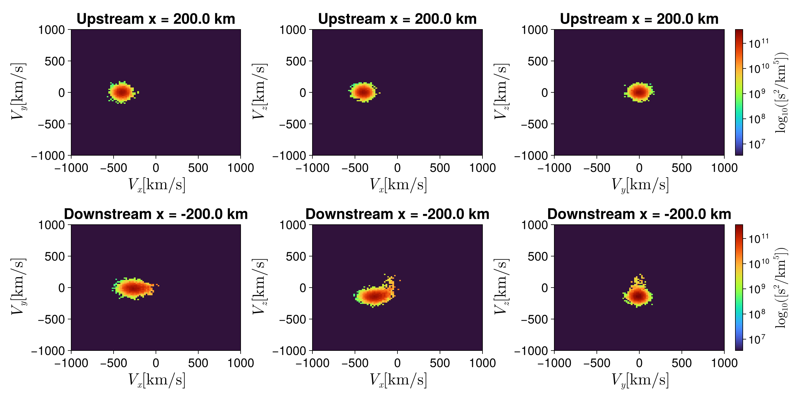
Each crossing contributes N and dv factors are absorbed in S, and the
Method 2: Forward Liouville tracking
Forward Liouville tracking starts from a sphere of initial conditions in velocity space at the source and traces forward to the detector. By Liouville's theorem
function reconstruct_liouville_projections(
        sols, detector, vdf, n0;
        dv_km = 20.0, vsphere = (4 / 3) * π * (vradius_m2 * 1.0e-3)^3
    )
    # Source f for every trajectory [s³/m⁶]
    ws0 = [n0 * pdf(vdf, s.u[1][SA[4, 5, 6]]) for s in sols.u]
    vxi = [s.u[1][4] for s in sols.u]
    # Detector crossings carry the source f (Liouville) together with the launch |v_x|
    vs, (ws, ws_vxi) = get_particle_crossings(sols, detector, (ws0, vxi))

    v_edges = -1000:dv_km:1000
    centers = bin_centers(v_edges)
    # Each sample stands for a source velocity volume `vsphere / N`, mapped onto the
    # detector and spread over the bin volume, so the bin density is Σ f·ΔV / dv³.
    # Summing keeps the `∝ 1/√n` counting noise; `average = true` divides it out instead.
    scale = vsphere * 1.0e18 / (length(sols.u) * dv_km^3) # [s³/m⁶] → [s³/km⁶]

    f_3d = bin_velocity_space(vs, ws .* scale, v_edges; vx_source = ws_vxi)
    f_xy, f_xz, f_yz = project_vdf(f_3d, dv_km)

    return ((centers, centers, f_xy), (centers, centers, f_xz), (centers, centers, f_yz))
end

nparticles_m2 = 100000
const vradius_m2 = 3 * vth_ion # velocity-space radius, [m/s]

# Uniform sampling in a 3D sphere
function prob_func_m2(prob, ctx)
    v = sample_velocity_ball(ctx.rng, vradius_m2; center = SA[V_sw, 0.0, 0.0])
    u0 = SA[x_source..., v...]
    return remake(prob, u0 = u0)
end

prob_m2 = TraceProblem(
    SA[0.0, 0.0, 0.0, 0.0, 0.0, 0.0], tspan, param; prob_func = prob_func_m2
)
t_liou = @elapsed sols_m2 = solve(
    prob_m2, Boris(), EnsembleThreads(); dt,
    trajectories = nparticles_m2, seed
);

hists_up_m2 = reconstruct_liouville_projections(sols_m2, detector_up, vdf, n_up)
hists_down_m2 = reconstruct_liouville_projections(sols_m2, detector_down, vdf, n_up)

fig_forward = plot_shock_vdf(hists_up_m2, hists_down_m2, x_upstream, x_downstream)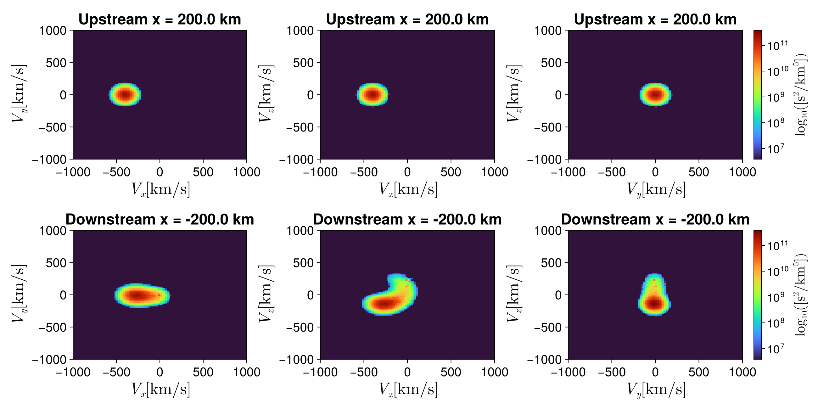
The sphere radius 3 vth_ion covers the bulk of the Maxwellian; nparticles_m2 = 10⁵ gives usable statistics in the populated bins. Note that the sharp circular boundary in the reconstructed phase-space plots is an artifact of the finite sampling sphere (r ≤ 3 vth_ion) at the source. The result is a direct Monte-Carlo estimate of
Method 3: Backward Liouville tracing
Starting from a velocity-space grid at the detector, each grid point is traced backward in time to the source plane. The phase-space density at the detector equals the source density evaluated at the traced-back state:
Every step is saved (the default) so that no source-plane crossing is missed, and a trajectory is terminated only once it has crossed the source plane and moved a safe distance beyond it (u[1] > x_source + margin). Gyrating trajectories that temporarily move away are not terminated, so every grid cell whose backward trajectory eventually crosses the source receives a value.
const source_plane = Meshes.Plane(Meshes.Point(x_source...), Meshes.Vec(1.0, 0.0, 0.0))

function reconstruct_backward_projections(
        detector_x, dt, param;
        v_range = 1000.0e3, vy_range = 1000.0e3, vz_range = 1000.0e3, dv_km = 20.0,
        adaptive = true, dv_coarse_km = 60.0, margin_km = 150.0
    )
    dv = dv_km * 1.0e3
    v0x = -v_range + dv / 2
    v0y = -vy_range + dv / 2
    v0z = -vz_range + dv / 2
    bounds = ((v0x, -v0x), (v0y, -v0y), (v0z, -v0z))

    t_solve = @elapsed begin
        f_3d_km, (vx_grid, vy_grid, vz_grid) = vdf_backward_trace(
            param, detector_x, source_plane, f_src;
            v_range, vy_range, vz_range, dv, dt, tspan = (0.0, -10.0),
            adaptive, dv_coarse = dv_coarse_km * 1.0e3, margin = margin_km * 1.0e3,
            relthresh = 1.0e-6, bounds,
            isoutside = (u, p, t) -> u[1] > x_source[1] + 100.0e3 ||
                u[1] < detector_x - 600.0e3
        )
    end
    nparticles_bw = length(vx_grid) * length(vy_grid) * length(vz_grid)

    f_xy, f_xz, f_yz = project_vdf(f_3d_km, dv_km)

    # `embed_vdf` places the sub-grid on the full grid by its step, so the centers
    # have to stay a range instead of a materialized vector.
    full_centers = range(v0x, -v0x; step = dv) .* 1.0e-3
    g1 = vx_grid .* 1.0e-3
    g2 = vy_grid .* 1.0e-3
    g3 = vz_grid .* 1.0e-3

    return (
            (full_centers, full_centers, embed_vdf(g1, g2, full_centers, f_xy)),
            (full_centers, full_centers, embed_vdf(g1, g3, full_centers, f_xz)),
            (full_centers, full_centers, embed_vdf(g2, g3, full_centers, f_yz)),
        ), t_solve, nparticles_bw
end

res_up_bw, t_bw_up, n_bw_up = reconstruct_backward_projections(x_upstream, dt, param)
res_down_bw, t_bw_down, n_bw_down = reconstruct_backward_projections(x_downstream, dt, param)
t_bw = t_bw_up + t_bw_down
n_bw = n_bw_up + n_bw_down

fig_backward = plot_shock_vdf(res_up_bw, res_down_bw, x_upstream, x_downstream)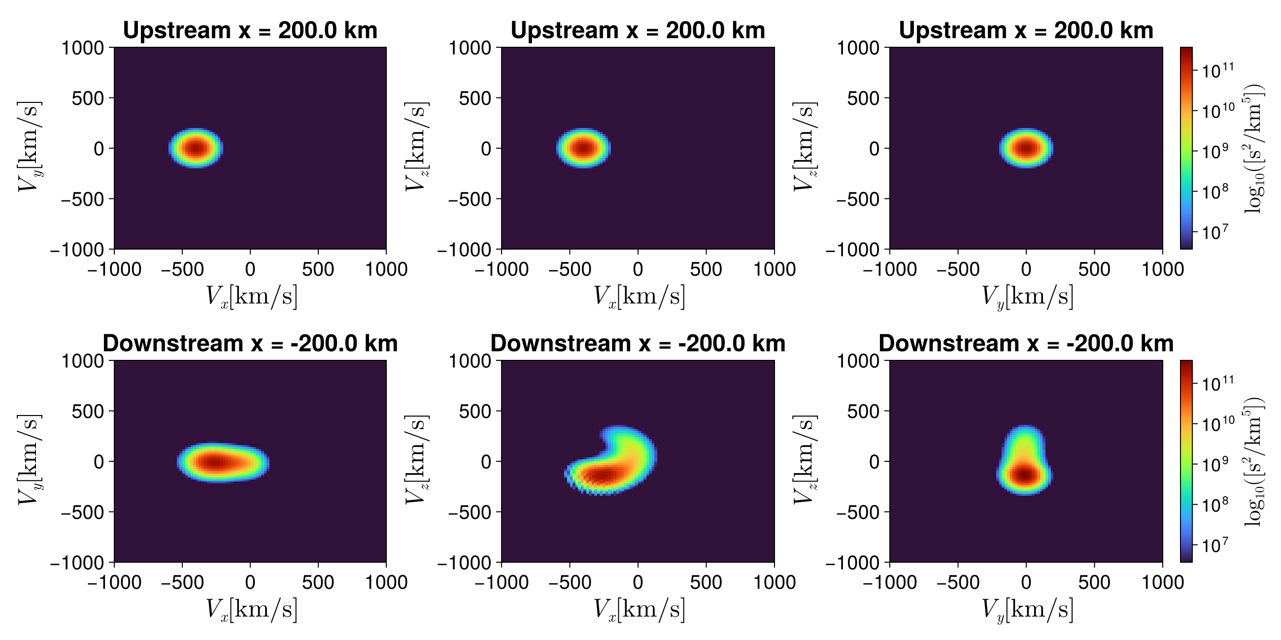
Comparison of the three methods (shared colour scale)
The downstream f from the three methods is compared using a single shared colour bar, so the colour ranges are directly comparable.
fig_cmp = plot_downstream_comparison(hists_down, hists_down_m2, res_down_bw)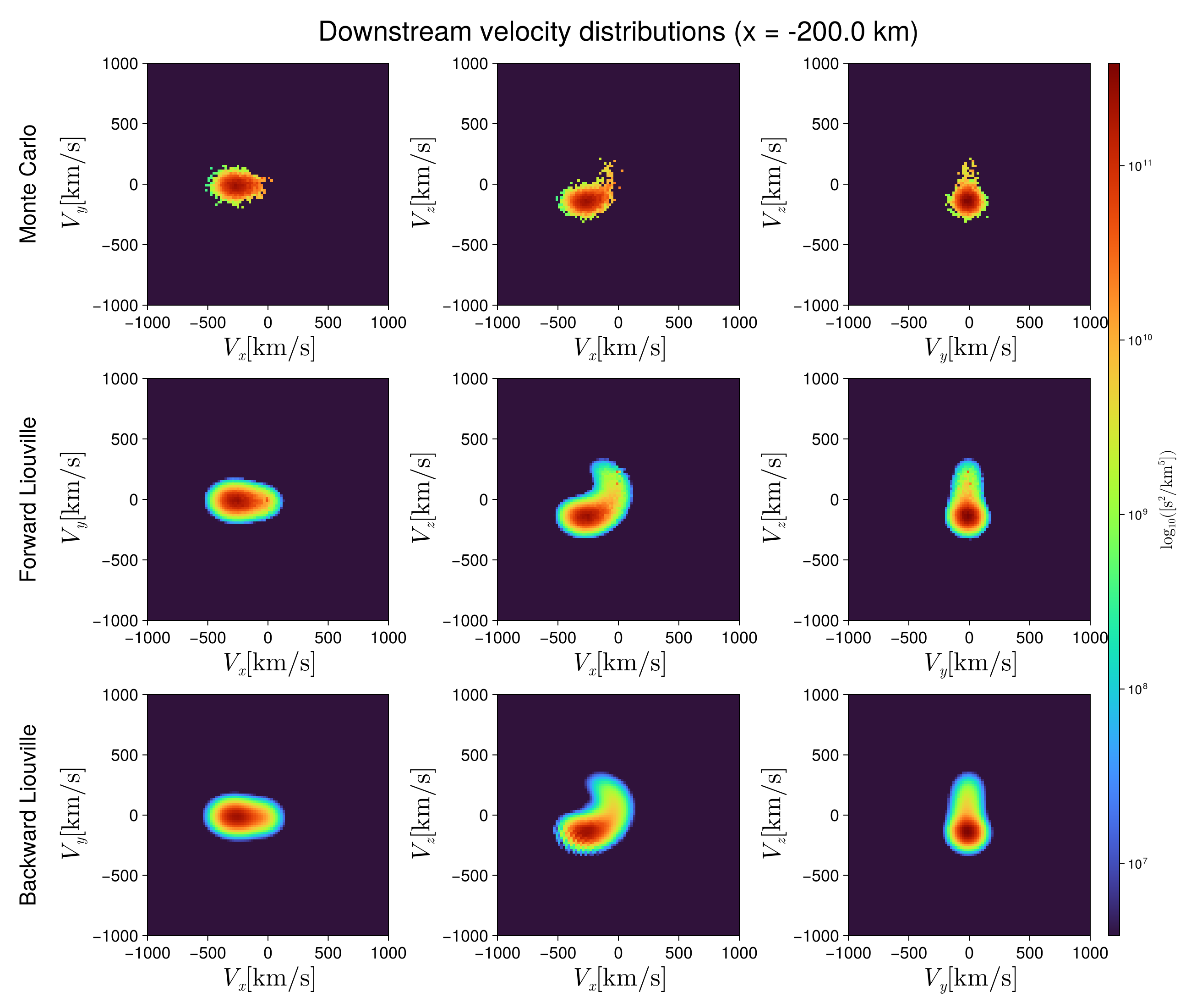
Validation
Moment check: density and momentum
Integrating a 2-D projection over velocity returns the lowest moments of the reconstructed distribution: the density
The three methods must agree with each other. They all reconstruct the same
in the same units, so their moments have to match; any mismatch is an error in the estimator rather than in the physics. Because the moments integrate the whole VDF, they are sensitive to normalisation errors and to repeated counting of the same trajectory, neither of which is obvious on a log colour scale. The upstream row is an absolute calibration. The upstream detector sits in the uniform, undisturbed solar wind, where the answer is known a priori:
The downstream row splits into one check that passes and one that cannot. Nothing is reflected at this Mach number and every ion crosses each detector plane exactly once, so the crossing-flux estimator carries no counting bias, and the momentum density does come out at the mass-flux value
. The density, however, lands near 4.9 instead of 6.0 [10⁶ m⁻³]: the transmitted beam arrives at ~250 km/s rather than the RH 200 km/s, because the prescribed fields can only decelerate the bulk through the electrostatic barrier discussed above. Read the downstream row as a statement about the model, not about the reconstruction.
| Method | n up [10⁶ m⁻³] | n·Vx up [10⁹ m⁻³·km/s] | n down [10⁶ m⁻³] | n·Vx down [10⁹ m⁻³·km/s] |
|---|---|---|---|---|
| Monte Carlo | 2.99 | -1.20 | 4.87 | -1.20 |
| Forward Liouville | 2.99 | -1.19 | 4.97 | -1.20 |
| Backward Liouville | 3.00 | -1.20 | 4.96 | -1.20 |
Accuracy and cost
The moments collapse each VDF into four numbers, so a wrong shape with the right normalisation and the wrong shape with the wrong normalisation can look identical to them. For a pointwise comparison we use the same relative L2 norm as the steady-state demo,
Upstream the reference can be exact: that plane still sees the undisturbed solar wind, and since vdf itself is the reference. Downstream no analytic reference exists, and the noise-free backward solution takes that role instead, so it is its own reference there and only the two forward methods get scored.
The last two rows are what each method needed to produce its
# Analytic references come out as bare matrices, while the reconstructions are
# `(vi, vj, f)` tuples; this normalizes both to the same matrix.
matrix_of(h::Tuple) = h[3]
matrix_of(M::AbstractMatrix) = M

const bin_edges = -1000.0:20.0:1000.0 # km/s, velocity bin edges of all three methods
const v_centers = bin_centers(bin_edges)
# Midpoint rule on the bin centers, i.e. the same quadrature the reconstructions use when
# they collapse the third velocity axis.
const v_int = range(-990.0, 990.0; step = 20.0) # km/s, integration axis

ana_up = (
    analytic_projection(f_src, 3, v_centers, v_centers, v_int, step(v_int)),
    analytic_projection(f_src, 2, v_centers, v_centers, v_int, step(v_int)),
    analytic_projection(f_src, 1, v_centers, v_centers, v_int, step(v_int)),
)

const recs_up = (hists_up, hists_up_m2, res_up_bw) # reconstructions at x_upstream
const recs_down = (hists_down, hists_down_m2) # forward reconstructions at x_downstream

const n_traj = (nparticles, nparticles_m2, n_bw) # trajectories behind each method
const t_cost = (t_mc, t_liou, t_bw) # wall-clock cost of each method [s]
cost = [
for i in 1:3| Quantity | Monte Carlo | Forward Liouville | Backward Liouville |
|---|---|---|---|
| Upstream rel. L2 error vs analytic solar wind, Vx–Vy | 0.091 | 0.065 | 0.000 |
| Downstream rel. L2 error vs backward Liouville, Vx–Vy | 0.144 | 0.099 | ref |
| Upstream rel. L2 error vs analytic solar wind, Vx–Vz | 0.077 | 0.080 | 0.000 |
| Downstream rel. L2 error vs backward Liouville, Vx–Vz | 0.175 | 0.152 | ref |
| Upstream rel. L2 error vs analytic solar wind, Vy–Vz | 0.084 | 0.058 | 0.000 |
| Downstream rel. L2 error vs backward Liouville, Vy–Vz | 0.105 | 0.085 | ref |
| Trajectories | 10000 | 100000 | 140822 |
| Wall-clock cost | 3.3 s (325.8 µs/traj) | 11.0 s (110.3 µs/traj) | 14.5 s (102.9 µs/traj) |
Summary
This example illustrates three complementary ways to reconstruct the phase-space density from particle simulations, all returning the same physical quantity