Relativistic vs Non-relativistic Tracing

This example compares the particle trajectories of trace! (non-relativistic) and trace_relativistic! (relativistic) solvers. We demonstrate two cases:

1. Uniform magnetic field (Cyclotron motion)

2. Uniform ExB field (ExB drift)

Relativistic effects become significant when the particle velocity approaches the speed of light . In the relativistic regime, the mass increases by a factor of  , leading to a larger gyroradius and different drift velocities compared to the classical prediction.

using TestParticle
using OrdinaryDiffEq
using StaticArrays
using CairoMakie

Case 1: Pure Magnetic Field (Cyclotron Motion)

We trace protons in a uniform magnetic field with varying initial velocities. Relativistic theory predicts a gyroradius   and gyrofrequency  . Non-relativistic theory predicts   and  .

Field and Particle Setup

const B0 = 1.0 # [T]
getB1(x) = SA[0.0, 0.0, B0]
getE1(x) = SA[0.0, 0.0, 0.0]

m = TestParticle.mᵢ
q = TestParticle.qᵢ
c = TestParticle.c

param = prepare(getE1, getB1; species = Proton);

Initial velocities to test: 10%, 50%, and 90% of speed of light

rats = [0.1, 0.5, 0.9]
v_ratios = [rat * c for rat in rats]
labels = ["0.1c", "0.5c", "0.9c"]
colors = [:darkcyan, :orange, :red];

Time span: enough for a few gyro-periods. Using the non-relativistic cyclotron period as a baseline reference.

Ω_non = q * B0 / m
T_non = 2π / Ω_non
tspan = (0.0, 4 * T_non);

Simulation and Plotting

f1 = Figure(size = (600, 600), fontsize = 20)
ax1 = Axis(
    f1[1, 1],
    title = "Trajectory comparison (XY plane)",
    xlabel = "x [m]", ylabel = "y [m]", aspect = DataAspect()
)

for (i, v_mag) in enumerate(v_ratios)
    # Let's start at same point (0,0,0) with v in x-dir.
    r0 = [0.0, 0.0, 0.0]
    v0 = [v_mag, 0.0, 0.0]

    # Non-relativistic initial state: [r, v]
    u0_non = [r0..., v0...]
    prob_non = ODEProblem(trace!, u0_non, tspan, param)
    sol_non = solve(prob_non, Vern7())

    # Relativistic initial state: [r, γv]
    γ = 1 / sqrt(1 - (v_mag / c)^2)
    u0_rel = [r0..., (γ * v0)...]
    prob_rel = ODEProblem(trace_relativistic!, u0_rel, tspan, param)
    sol_rel = solve(prob_rel, Vern7())

    # Plot
    lines!(
        ax1, sol_non; idxs = (1, 2), linestyle = :dash,
        color = colors[i], label = "Non-rel $(labels[i])"
    )
    lines!(
        ax1, sol_rel; idxs = (1, 2), linestyle = :solid,
        color = colors[i], label = "Rel $(labels[i])"
    )
end

axislegend(ax1; position = :rt, backgroundcolor = :transparent)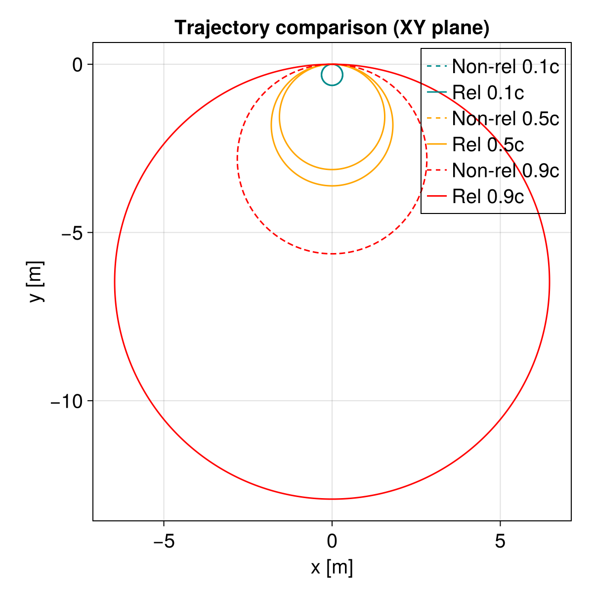

Observation: At 0.1c, the dashed and solid lines almost overlap. At 0.9c, the relativistic trajectory (solid) has a significantly larger radius, consistent with the factor of γ ≈ 2.29 increase in effective mass.

Case 2: ExB Drift

We add a uniform electric field . The drift velocity is given by  . However, relativistic drift must satisfy   (or strictly speaking, in the drift frame). The relativistic drift velocity matches the non-relativistic form   only if we consider the cross-field velocity. But the particle mass dilation affects the gyroradius superimposed on this drift. Actually, there is a relativistic limit where if  , the particle is accelerated continuously. We will choose such that  .

const E0 = 0.5 * c * B0 # strong electric field, v_drift = 0.5c
getB2(x) = SA[0.0, 0.0, B0]
getE2(x) = SA[0.0, E0, 0.0]

param2 = prepare(getE2, getB2; species = Proton);

Test with a single high initial velocity perpendicular to drift to see the cycloid differences. Starting from rest: Non-relativistic: cycloid with peak velocity 2*v_drift. Relativistic: should also drift but with different dynamics.

v_init_mag = 0.0 # start from rest
r0 = [0.0, 0.0, 0.0]
v0 = [0.0, v_init_mag, 0.0];

Non-relativistic

u0_non = [r0..., v0...]
prob_non_drift = ODEProblem(trace!, u0_non, tspan, param2)
sol_non_drift = solve(prob_non_drift, Vern7());

Relativistic if v=0, γ=1

u0_rel = [r0..., v0...]
prob_rel_drift = ODEProblem(trace_relativistic!, u0_rel, tspan, param2)
sol_rel_drift = solve(prob_rel_drift, Vern7());

Trajectory comparison

f2 = Figure(size = (1000, 300), fontsize = 20)
ax2 = Axis(
    f2[1, 1],
    title = "ExB Drift comparison (XY plane)",
    xlabel = "x [m]", ylabel = "y [m]", aspect = DataAspect()
)

lines!(
    ax2, sol_non_drift; idxs = (1, 2), linestyle = :dash,
    color = :darkcyan, label = "Non-rel drift"
)
lines!(
    ax2, sol_rel_drift; idxs = (1, 2), linestyle = :solid,
    color = :darkorange, label = "Rel drift"
)

axislegend(ax2; position = :rb, backgroundcolor = :transparent)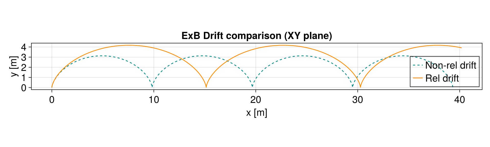

Summary

• Case 1: Relativistic particles have larger gyroradii due to the relativistic factor .

• Case 2: Under strong electric fields, relativistic kinematics limit the velocity to , whereas non-relativistic dynamics would predict velocities exceeding (if is large enough or during the gyro-phase).