Cosmic Ray Propagation

This example shows how to trace cosmic rays in a turbulent magnetic field. Everything is dimensionless and normalized following Cosmic ray propagation in sub-Alfvénic magnetohydrodynamic turbulence. The general dimensionless-unit and SI↔dimensionless normalization (including relativistic tracing and periodic boundaries) is covered in the Dimensionless Units and Normalization example; here we use the cosmic-ray-specific form of that normalization.

With     a particle of perpendicular velocity in a local field has gyroradius

so one unit of distance equals one gyroradius. We trace with two solvers that share the same underlying physics: the classic ODE (Runge–Kutta, ) and the native Boris pusher ( through the ensemble interface). The latter is the same solver path used for production runs on MHD snapshots; the only difference is that the field is loaded from HDF5 instead of generated synthetically. We verify below that both solvers produce consistent results.

using TestParticle, StaticArrays, LinearAlgebra, Random, Statistics
import TestParticle as TP
using OrdinaryDiffEq
using CairoMakie

1. Cosmic-ray normalization

Each particle of charge and mass has momentum   and propagates in (no mean electric field) and   . The particle is injected with a Lorentz factor that sets its initial Larmor radius

where is the background field strength. The synchrotron pulsation is   (a gyro-frequency in the particle's own frame); a particle with pitch-angle cosine    completes one orbit in time.

After normalization, with the velocity normalized by , the electric field by , the magnetic field by , the position by , and the time by , the equations become

where  . In the interstellar medium the electric field is negligible for high-energy (multi-TeV) cosmic rays, energy is conserved, and  . The equations simplify to

The factor is removed by rescaling the position with , giving simply   (the domain extent becomes ). Taking      then yields   and  .

The ratio controls how many discrete grid points fall within one gyroradius. The smaller is, the more inhomogeneous the field is during a single gyration, and the more strongly the particle is scattered. With   the perpendicular and parallel speeds are   and  .

2. Magnetic fields

We use a uniform field for the single-particle sanity check, and a synthetic guide field plus transverse Fourier modes for the ensemble. The synthetic field mirrors a production run, where would be an MHD snapshot interpolated with TP.build_interpolator(F, gridx, gridy, gridz, 1, TP.WrapExtrap()) and normalized by so that the background guide field is 1.

B0 = 1.0
B_uniform(x) = SA[0.0, 0.0, B0]
E_zero(x) = SA[0.0, 0.0, 0.0]

param_uniform = prepare(E_zero, B_uniform; q = 1.0, m = 1.0)

function generate_turbulent_field(
        gridx, gridy, gridz; B0 = 1.0, amp = 0.3, n_modes = 6, kmax = 3, seed = 42
    )
    nx, ny, nz = length(gridx), length(gridy), length(gridz)
    F = zeros(3, nx, ny, nz)
    F[3, :, :, :] .= B0
    rng = MersenneTwister(seed)
    for _ in 1:n_modes
        k = rand(rng, -kmax:kmax, 3)
        while all(k .== 0)
            k = rand(rng, -kmax:kmax, 3)
        end
        phase = 2π * rand(rng)
        a = amp * randn(rng)
        for i in 1:nx, j in 1:ny, kk in 1:nz
            s = k[1] * gridx[i] + k[2] * gridy[j] + k[3] * gridz[kk] + phase
            F[1, i, j, kk] += a * cos(s)
            F[2, i, j, kk] += a * sin(s)
        end
    end
    return F
end

nx = ny = nz = 24
dx = 0.5
L = nx * dx
gridx = range(dx / 2, L - dx / 2; length = nx)
gridy = range(dx / 2, L - dx / 2; length = ny)
gridz = range(dx / 2, L - dx / 2; length = nz)

F = generate_turbulent_field(gridx, gridy, gridz; B0)
itp = TP.build_interpolator(F, gridx, gridy, gridz, 1, TP.WrapExtrap())
Bfunc(x) = itp(x) ./ B0 # normalize: background guide field -> 1

param = prepare(E_zero, Bfunc; q = 1.0, m = 1.0);

3. Solver consistency: trace_normalized! vs Boris

Both solvers advance the same normalized equations   ,   with the same param (and therefore the same field evaluation). We check that they agree.

3.1 Uniform field: both give a circle of radius 1

A particle launched with   perpendicular to   executes a circle of radius   . We trace it with the RK solver and the Boris solver and overlay the orbits.

stateinit = [0.0, 0.0, 0.0, 1.0, 0.0, 0.0] # v = 1 -> r_L = 1
tspan0 = (0.0, 2π)

prob_rk = ODEProblem(trace_normalized!, stateinit, tspan0, param_uniform)
sol_rk = solve(prob_rk, Vern9(); reltol = 1.0e-9, abstol = 1.0e-11)

prob_b = TraceProblem(stateinit, tspan0, param_uniform)
sol_b = solve(
    prob_b, TP.MultistepBoris4(n = 4);
    dt = 2π / 40
);

The initial gyroradius from each solver (computed at the final state) should be ~1.

function rL_of(sol, Bfunc)
    xv = sol isa AbstractVector ? sol : sol.u[end]
    x = xv[SA[1, 2, 3]]; v = xv[SA[4, 5, 6]]
    B = Bfunc(x); Bmag = norm(B); b̂ = B ./ Bmag
    vpar = b̂ ⋅ v; vperp = v - vpar * b̂
    return norm(vperp) / Bmag
end
println("r_L (RK)  = ", round(rL_of(sol_rk, B_uniform); digits = 4))
println("r_L (Boris) = ", round(rL_of(sol_b, B_uniform); digits = 4))

f = Figure(fontsize = 18)
ax = Axis(
    f[1, 1], title = "Perpendicular orbit (r_L = 1): both solvers",
    xlabel = "X", ylabel = "Y", aspect = DataAspect()
)
lines!(ax, sol_rk, idxs = (1, 2); color = :steelblue, linewidth = 2, label = "RK (trace_normalized!)")
lines!(ax, sol_b[1, :], sol_b[2, :]; color = :tomato, linestyle = :dash, linewidth = 2, label = "Boris")
axislegend(ax)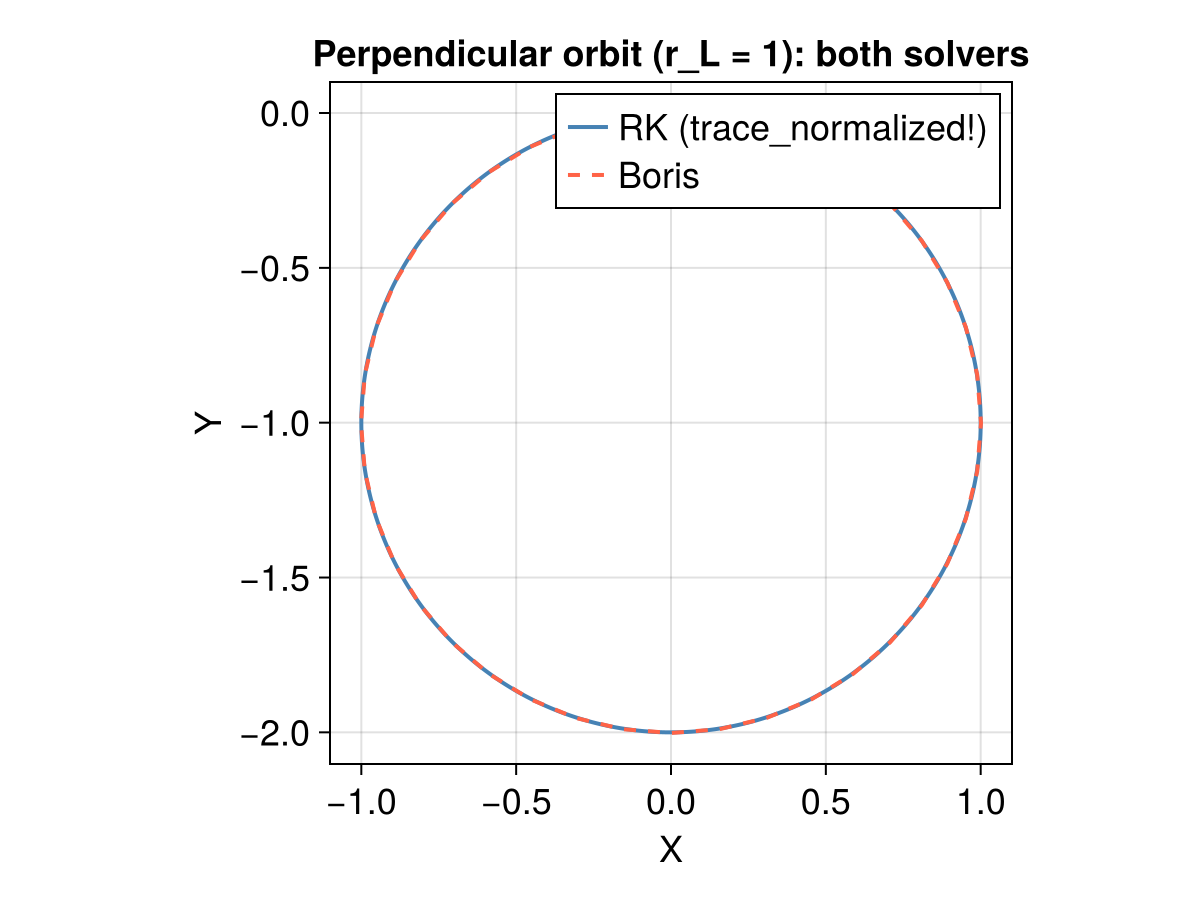

3.2 Turbulent field: single particle, both solvers

We now inject one particle into the synthetic turbulent field and integrate a few gyroperiods with both solvers, using the identical initial state and param. We overlay the X–Y projections and report the maximum separation relative to the gyroradius — it is tiny, confirming the solvers agree.

x0 = SA[0.5L, 0.5L, 0.5L]
Bv = Bfunc(x0); b0 = normalize(Bv)
e1 = SA[0.0, -b0[3], b0[2]]
e1 = norm(e1) > 1.0e-8 ? normalize(e1) : SA[0.0, 1.0, 0.0]
v0 = e1 + 0.3 * b0                 # |v| ≈ 1, mostly perpendicular
stateinit_t = collect(vcat(x0, v0))
tspan_t = (0.0, 2π * 3)

prob_rk_t = ODEProblem(trace_normalized!, stateinit_t, tspan_t, param)
sol_rk_t = solve(prob_rk_t, Vern9(); reltol = 1.0e-9, abstol = 1.0e-11)

prob_b_t = TraceProblem(stateinit_t, tspan_t, param)
sol_b_t = solve(
    prob_b_t, TP.MultistepBoris4(n = 4);
    dt = 2π / 80, trajectories = 1
)

trange = range(tspan_t..., length = 201)
rk_xy = [sol_rk_t(t)[SA[1, 2]] for t in trange]
bc_xy = [sol_b_t(t)[SA[1, 2]] for t in trange]
sep = maximum(norm(sol_rk_t(t)[SA[1, 2, 3]] - sol_b_t(t)[SA[1, 2, 3]]) for t in trange)
println("Max position separation / r_L0 (turbulent, 3 gyroperiods) = ", round(sep; digits = 4))
@assert sep < 0.2 "RK and Boris solvers disagree unexpectedly (sep = $sep)"

f = Figure(fontsize = 18)
ax = Axis(
    f[1, 1], title = "Turbulent-field trajectory: both solvers",
    xlabel = "X", ylabel = "Y", aspect = DataAspect()
)
lines!(ax, first.(rk_xy), last.(rk_xy); color = :steelblue, linewidth = 2, label = "RK (trace_normalized!)")
lines!(ax, first.(bc_xy), last.(bc_xy); color = :tomato, linestyle = :dash, linewidth = 2, label = "Boris")
axislegend(ax)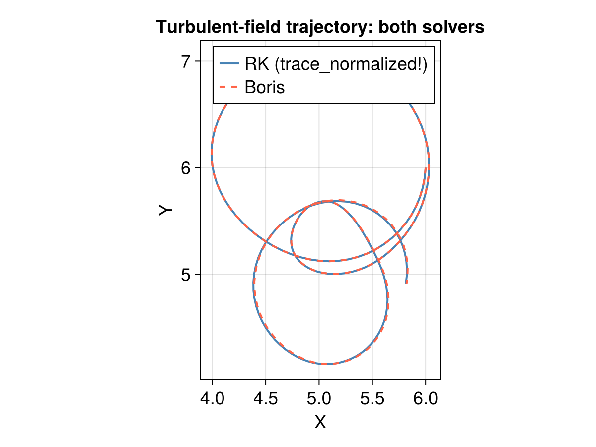

4. Constant-initial-gyroradius injection

The key physics choice for an energy scan: we fix the initial gyroradius rather than the initial speed. Because  , we scale the perpendicular speed by the local field magnitude,

where   is the initial pitch-angle cosine. With this convention the injected gyroradius is identical for every particle and every guide-field snapshot, so different energies are directly comparable.

prob_func receives (prob, ctx) where ctx.rng is a per-trajectory RNG, and returns a remaked problem with the new initial state.

function make_injection(Lx, Ly, Lz; rL = 1.0)
    function prob_func(prob, ctx)
        r = rand(ctx.rng, 5)
        x = Lx * (0.1 + 0.8 * r[1])
        y = Ly * (0.1 + 0.8 * r[2])
        z = Lz * (0.1 + 0.8 * r[3])
        loc = SA[x, y, z]

        Bvec = prob.p[4](loc)
        Bmag = norm(Bvec)
        b0 = Bvec ./ Bmag

        bperp1 = SA[0.0, -b0[3], b0[2]]
        n1 = norm(bperp1)
        bperp1 = n1 > 1.0e-8 ? bperp1 ./ n1 : SA[0.0, 1.0, 0.0]
        bperp2 = b0 × bperp1 |> normalize
        bperp1 = bperp2 × b0

        ϕ = 2π * r[4]
        μ0 = 0.999 * r[5]          # pitch-angle cosine in [0, 1)
        sinα = √(1 - μ0^2)
        sinϕ, cosϕ = sincos(ϕ)

        vperp_mag = rL * Bmag
        vperp = (bperp1 .* cosϕ .+ bperp2 .* sinϕ) .* vperp_mag
        vpar_mag = vperp_mag * μ0 / sinα
        v0 = vpar_mag .* b0 .+ vperp

        return remake(prob; u0 = [x, y, z, v0...])
    end
    return prob_func
end

make_injection (generic function with 1 method)

5. Ensemble tracing (Boris)

We trace a small ensemble with MultistepBoris4 (4th-order gyrophase correction, 4 subcycles). In production this is where you would loop over the energy (rL) and pitch-angle (μ0) bins and the guide-field snapshots, writing each trajectory to a JLD2 file via save_output.

rL0 = 1.0
tspan = (0.0, 2π * 150)
prob_func = make_injection(L, L, L; rL = rL0)
prob = TraceProblem(stateinit, tspan, param; prob_func)

alg = TP.MultistepBoris4(n = 4)
dt = 2π / 40
sols = solve(
    prob, alg, EnsembleThreads();
    dt, saveat = 15 * dt, trajectories = 32, seed = 1234
);

6. Analysis

6.1 Trajectories, guiding center, and phase-space evolution

We plot a few trajectories together with their guiding centers (computed with get_gc_func), and for one trajectory show how the gyroradius and pitch-angle cosine evolve. The gyroradius starts at and then drifts as the particle samples regions of different and is scattered.

gc = param |> get_gc_func

f = Figure(fontsize = 16, size = (700, 500))
ax = Axis3(f[1, 1], title = "Sample trajectories and guiding centers", aspect = :data)

for (i, sol) in enumerate(sols.u[1:4])
    x = sol[1, :]; y = sol[2, :]; z = sol[3, :]
    lines!(ax, x, y, z; color = Makie.wong_colors()[i], linewidth = 1.5)
    gcx = [gc(sol.u[k])[1] for k in eachindex(sol.u)]
    gcy = [gc(sol.u[k])[2] for k in eachindex(sol.u)]
    gcz = [gc(sol.u[k])[3] for k in eachindex(sol.u)]
    lines!(ax, gcx, gcy, gcz; color = Makie.wong_colors()[i], linestyle = :dash)
end

function phase_evolution(sol, Bfunc)
    n = length(sol.u)
    t = sol.t
    ρ = zeros(n)
    μ = zeros(n)
    for k in 1:n
        x = sol.u[k][SA[1, 2, 3]]
        v = sol.u[k][SA[4, 5, 6]]
        B = Bfunc(x)
        Bmag = norm(B)
        b̂ = B ./ Bmag
        vpar = b̂ ⋅ v
        vperp = v - vpar * b̂
        ρ[k] = norm(vperp) / Bmag
        μ[k] = vpar / norm(v)
    end
    return t, ρ, μ
end

t1, ρ1, μ1 = phase_evolution(sols.u[1], Bfunc)

f = Figure(fontsize = 16, size = (1000, 600))
axρ = Axis(f[1, 1], xlabel = "t / 2π", ylabel = L"r_L")
axμ = Axis(f[2, 1], xlabel = "t / 2π", ylabel = "μ")
lines!(axρ, t1 ./ (2π), ρ1; color = :steelblue, label = L"r_L")
hlines!(axρ, [rL0]; color = :tomato, linestyle = :dash)
lines!(axμ, t1 ./ (2π), μ1; color = :seagreen, label = "μ")
axislegend(axρ); axislegend(axμ)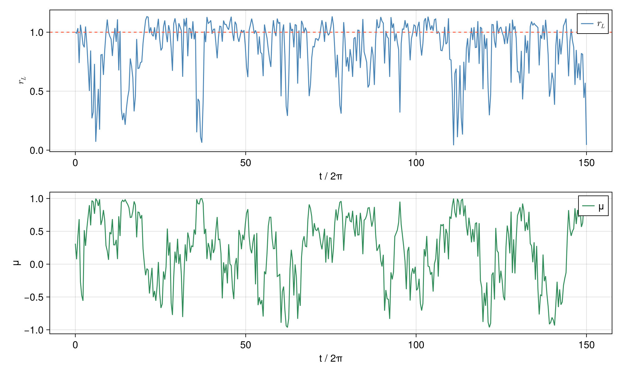

6.2 Energy scan: diffusion grows with gyroradius

Sweep over the initial gyroradius . We compute the ensemble-mean squared displacement as a function of time for several energies. Higher-energy (larger ) particles sample more field modes per gyro-orbit and diffuse faster.

rL_list = [0.5, 1.0, 2.0]
colors = Makie.wong_colors()

f = Figure(fontsize = 18, size = (1000, 600))
ax = Axis(
    f[1, 1], xlabel = "t / 2π", ylabel = "⟨|Δx|²⟩",
    title = "Mean squared displacement vs initial gyroradius"
)

for (j, rL) in enumerate(rL_list)
    pfunc = make_injection(L, L, L; rL)
    pscan = TraceProblem(stateinit, (0.0, 2π * 100), param; prob_func = pfunc)
    dt = 2π / 40
    ssols = solve(
        pscan, alg, EnsembleThreads();
        dt, saveat = 10 * dt, trajectories = 16, seed = 1234
    )
    nt = length(ssols.u[1].u)
    msr = zeros(nt)
    for sol in ssols.u
        r0 = sol.u[1][SA[1, 2, 3]]
        for k in 1:nt
            Δ = sol.u[k][SA[1, 2, 3]] - r0
            msr[k] += Δ ⋅ Δ
        end
    end
    msr ./= length(ssols.u)
    lines!(ax, ssols.u[1].t ./ (2π), msr; label = "r_L0 = $rL", color = colors[j])
end
axislegend(ax; position = :lt)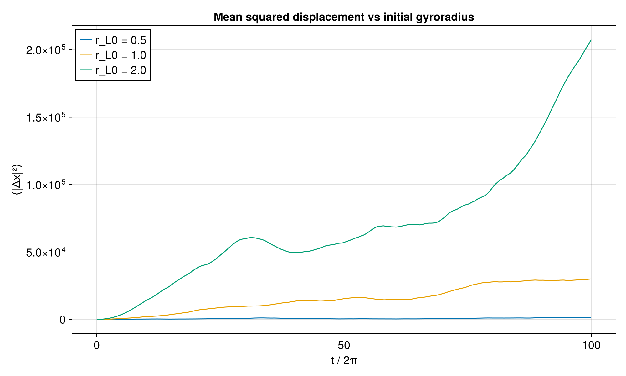

7. Production notes

For a real run you would replace the synthetic field with a snapshot loaded from disk and write the output to disk. The workflow maps as follows:

• load_B(filedir, idx) / load_J(...) → an F array (3×nx×ny×nz).

• TP.build_interpolator(F, gridx, gridy, gridz, 1, TP.WrapExtrap()) ./ B0 builds the periodic, normalized field.

• The prob_func above is unchanged — it already scales by the local so the injected is identical across snapshots and energies.

• After tracing, save per-trajectory diagnostics (guiding center, , current density , curvature via TP.get_magnetic_properties) to JLD2, mirroring the production save_output.