Tokamak Configurations

Tokamak Coils

Magnetic field from a Tokamak topology consisting of $N$ toroidal field coils and a plasma current. The total field is the sum of contributions from all coils and the plasma ring:

$$\mathbf{B}(\mathbf{r})=\sum _{i=1}^N{\mathbf{B}}_{\text{coil},i}(\mathbf{r})+{\mathbf{B}}_{\text{plasma}}(\mathbf{r})$$

using Magnetostatics, StaticArrays, LinearAlgebra
using CairoMakie

a = 1.0  # Coil radius
b = 2.0  # Major radius offset
ICoils = 1000.0
IPlasma = 500.0

# Query point
x, y, z = 3.0, 0.0, 0.0
B = getB_tokamak_coil(x, y, z, a, b, ICoils, IPlasma)
println("B at ($x, $y, $z): $B [T]")

B at (3.0, 0.0, 0.0): [-1.3552527156068805e-20, 0.0010636276263681892, 0.00013054917085968874] [T]

Visualizing the poloidal field (xz-plane):

xs = range(0.5, 4.5, length=51)
zs = range(-2, 2, length=51)

function field_xz_tokamak(x, z)
    B = getB_tokamak_coil(x, 0.0, z, a, b, ICoils, IPlasma)
    return Point2f(B[1], B[3])
end

Bmag = [norm(getB_tokamak_coil(x, 0.0, z, a, b, ICoils, IPlasma)) for x in xs, z in zs]

fig = Figure(size = (700, 600), fontsize=20)
ax = Axis(fig[1, 1];
    xlabel="x (R)", ylabel="z", aspect=DataAspect(), title="Tokamak Coil Field (Poloidal)")

hm = heatmap!(ax, xs, zs, log10.(Bmag .+ 1e-9), colormap=:plasma)
Colorbar(fig[1, 2], hm, label="log10(|B|)")

streamplot!(ax, field_xz_tokamak, xs[1]..xs[end], zs[1]..zs[end];
    arrow_size = 8, linewidth = 1.5)

fig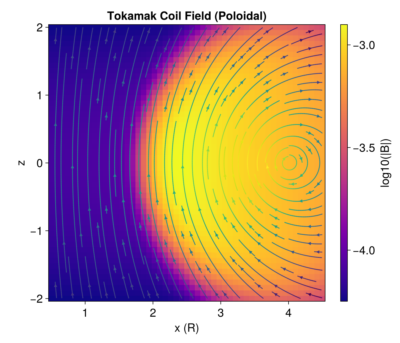

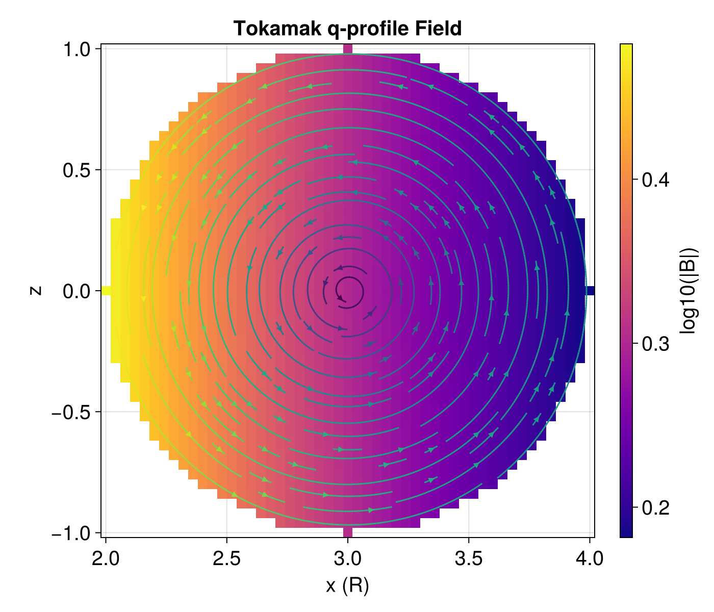
Tokamak with q-profile

Reconstruct the magnetic field distribution from a safety factor ($q$) profile. The magnetic field components in local cylindrical coordinates $(R,\zeta ,z)$ relative to the major radius $R_0$ and minor radius $r$ are given by:

$$\begin{array}{rl}{B}_{\zeta }& =B_{\zeta 0}\frac{R_0}{R}\\ B_{\theta }& =\frac{r{B}_{\zeta }}{R_{0}q(r/a)}\end{array}$$

where $B_{\zeta 0}$ is the toroidal field on axis, $q(r/a)$ is the safety factor profile, and $\theta$ is the poloidal angle.

using Magnetostatics, StaticArrays, LinearAlgebra
using CairoMakie

# Define q-profile as a function of normalized radius r/a
q_profile(r_norm) = 1.1 + r_norm^2

a = 1.0   # Minor radius
R0 = 3.0  # Major radius
B0 = 2.0  # Toroidal field on axis

# Query point inside plasma
x, y, z = 3.5, 0.0, 0.0
B = getB_tokamak_profile(x, y, z, q_profile, a, R0, B0)
println("B at ($x, $y, $z): $B [T]")

B at (3.5, 0.0, 0.0): [-0.0, 1.7142857142857142, 0.2116402116402116] [T]

Visualizing the q-profile field:

xs = range(R0 - a, R0 + a, length=51)
zs = range(-a, a, length=51)

function field_xz_tokamak_q(x, z)
    # Check if inside plasma
    r_local = sqrt((x - R0)^2 + z^2)
    if r_local > a
        return Point2f(NaN, NaN)
    end
    B = getB_tokamak_profile(x, 0.0, z, q_profile, a, R0, B0)
    return Point2f(B[1], B[3])
end

# Check if inside plasma
function get_Bmag_tokamak_q(x, z)
    if sqrt((x - R0)^2 + z^2) > a
        return NaN
    end
    return norm(getB_tokamak_profile(x, 0.0, z, q_profile, a, R0, B0))
end
Bmag = [get_Bmag_tokamak_q(x, z) for x in xs, z in zs]

fig = Figure(size = (700, 600), fontsize=20)
ax = Axis(fig[1, 1];
    xlabel="x (R)", ylabel="z", aspect=DataAspect(), title="Tokamak q-profile Field")

hm = heatmap!(ax, xs, zs, log10.(Bmag .+ 1e-9), colormap=:plasma)
Colorbar(fig[1, 2], hm, label="log10(|B|)")

streamplot!(ax, field_xz_tokamak_q, xs[1]..xs[end], zs[1]..zs[end];
    arrow_size = 8, linewidth = 1.5)
fig