Poisson Solver

The magnetostatic vector potential satisfies the Poisson equation

$${\mathrm{\nabla }}^2\mathbf{A}=-{\mu }_0\mathbf{J},$$

where $\mathbf{A}$ is related to the magnetic field via $\mathbf{B}=\mathrm{\nabla }\times \mathbf{A}$. The three Cartesian components of $\mathbf{A}$ decouple into independent scalar Poisson problems solved on a Cartesian grid using a sparse 7-point finite-difference Laplacian with homogeneous Dirichlet boundary conditions ($\mathbf{A}=0$ at domain faces). Each axis may have a different spacing ($\mathrm{\Delta }x$, $\mathrm{\Delta }y$, $\mathrm{\Delta }z$); the solver derives these automatically from the grid ranges passed to PoissonSolver.

PoissonSolver wraps any LinearSolve.jl algorithm. The default is the iterative conjugate-gradient (KrylovJL_CG), while sparse-direct factorizations such as KLUFactorization are also supported.

Infinite Wire — Comparing Direct and Krylov Solvers

We deposit a finite current-carrying wire along the z-axis onto a grid and solve for $A_z$ with both a direct and an iterative solver, then compare.

using Magnetostatics, StaticArrays, LinearSolve
import Magnetostatics as MS
using CairoMakie

Nx, Ny, Nz = 64, 64, 4
L = 2.0   # domain half-width [m], same for all axes

# Each axis spans the full domain [-L, L) with its own resolution:
# dx = dy = 2L/64 ≈ 0.0625 m, dz = 2L/8 = 0.5 m  (8× coarser in z)
xs = range(-L, L; length = Nx + 1)[1:end-1]
ys = range(-L, L; length = Ny + 1)[1:end-1]
zs = range(-L, L; length = Nz + 1)[1:end-1]
dx, dy, dz = step(xs), step(ys), step(zs)

# Deposit a Gaussian-profiled wire along z at the domain center
I_wire = 1.0
width  = 3dx   # Gaussian half-width based on xy resolution
J = zeros(Float64, 3, Nx, Ny, Nz)
set_current_wire!(J, xs, ys, zs, SVector(0.0, 0.0, 0.0), SVector(0.0, 0.0, 1.0), I_wire, width)

# Direct solver (sparse LU via KLU)
A_direct = MS.solve(PoissonSolver(xs, ys, zs; alg = KLUFactorization()), J)

# Iterative solver (conjugate gradient)
A_cg = MS.solve(PoissonSolver(xs, ys, zs; alg = KrylovJL_CG()), J)

println("Max |A_direct - A_cg| / max|A_direct| = ",
    maximum(abs, A_direct .- A_cg) / maximum(abs, A_direct))

Max |A_direct - A_cg| / max|A_direct| = 3.021362620558843e-5

Both solvers produce the same result. The midplane slice of $A_z$ shows the expected bell-shaped peak centred on the wire:

ic = Nz ÷ 2 + 1 # index closest to grid center

fig = Figure(size = (650, 500), fontsize = 18)
ax = Axis(fig[1, 1];
    xlabel = "x [m]", ylabel = "y [m]",
    aspect = DataAspect(),
    title = "Az midplane (z-wire, Dirichlet BC)")

Az_mid = A_direct[3, :, :, ic]
hm = heatmap!(ax, xs, ys, Az_mid; colormap = :inferno)
Colorbar(fig[1, 2], hm; label = "Az [T·m]")
fig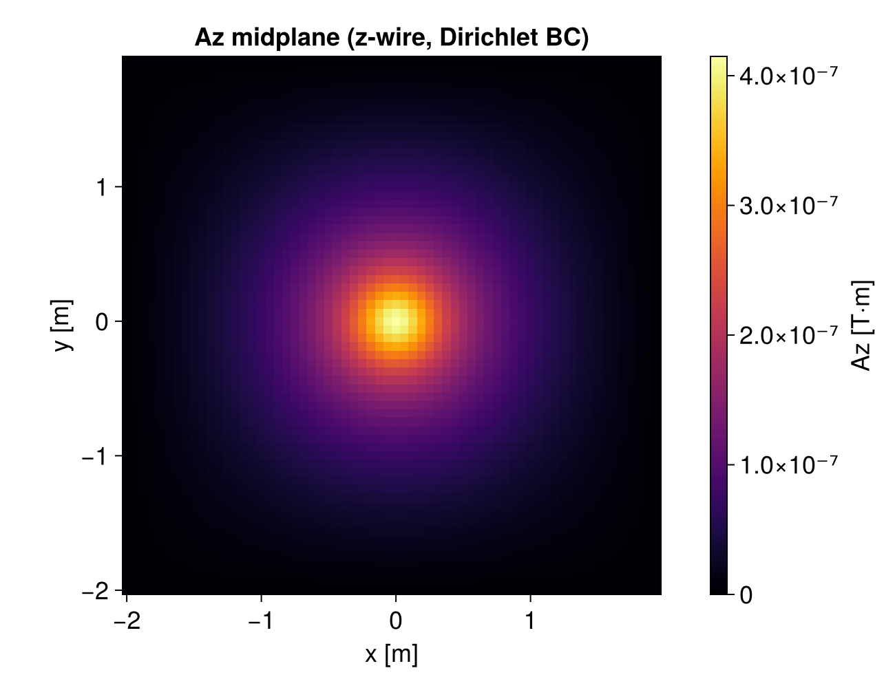

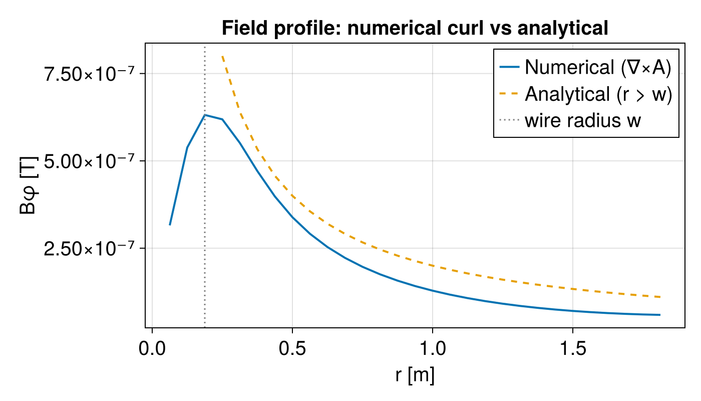
Recovering B = ∇ × A via Central Differences

After solving for $\mathbf{A}$ we can numerically recover $\mathbf{B}$ and compare it against the analytical solution for an infinite straight wire:

$$B_{\varphi }(r)=\frac{{\mu }_{0}I}{2\pi r}$$

Two sources of discrepancy are expected and are not a sign of grid coarseness:

• Inside the Gaussian core ($r<w$): the current is deposited with a Gaussian profile of half-width $w$ (width = 3dx), not on an infinitely thin wire. Inside the wire the field peaks at a finite value and falls to zero at $r=0$, whereas the thin-wire formula diverges. The analytical formula is valid only for $r>w$.

• Near the domain boundary ($r\to L$): the Dirichlet BCs force $\mathbf{A}=0$ at the box faces, suppressing $\mathbf{A}$ — and hence the curl — below the free-space value. This is a finite-box artefact, independent of grid resolution.

using LinearAlgebra

B_num = zeros(3, Nx, Ny, Nz)
compute_curl!(B_num, A_direct, xs, ys, zs)

# Radial profile along positive x-axis (y = 0, z = midplane)
jc    = Ny ÷ 2 + 1            # y-midplane index
ir    = ic                    # z-midplane index
i_pos = (Nx ÷ 2 + 2):(Nx - 2) # indices where xs[i] > 0
rs_num = xs[i_pos]
Bφ_num = [norm(SVector(B_num[1, i, jc, ir], B_num[2, i, jc, ir])) for i in i_pos]

# Analytical formula valid only outside the Gaussian core (r > width)
rs_ana = filter(>(width), rs_num)
Bφ_ana = MS.μ₀ * I_wire ./ (2π .* rs_ana)

fig2 = Figure(size = (700, 400), fontsize = 20)
ax2  = Axis(fig2[1, 1];
    xlabel = "r [m]", ylabel = "Bφ [T]",
    title  = "Field profile: numerical curl vs analytical")

lines!(ax2, rs_num, Bφ_num;
    label = "Numerical (∇×A)", linewidth = 2)
lines!(ax2, rs_ana, Bφ_ana;
    label = "Analytical (r > w)", linewidth = 2, linestyle = :dash)
vlines!(ax2, [width];
    color = :gray, linestyle = :dot, linewidth = 1.5, label = "wire radius w")
axislegend(ax2; position = :rt)
fig2