Current Sheets

Various current sheet models used in space physics and plasma physics.

Harris Sheet

A current sheet model often used in space physics, described by the exact field:

$$\mathbf{B}(z)=B_0\tanh \left(\frac{z}{L}\right)\hat{x}$$

where $B_0$ is the asymptotic magnetic field strength and $L$ is the half-width of the current sheet.

using Magnetostatics, StaticArrays, LinearAlgebra
using CairoMakie

B0 = 1.0       # Asymptotic field strength
L = 2.0        # Half-width
sheet = HarrisSheet(B0, L)

r = SVector(0.0, 0.0, 1.0)
B = sheet(r)
println("B at $r: $B [T]")

B at [0.0, 0.0, 1.0]: [0.46211715726000974, 0.0, 0.0] [T]

xs = range(-5, 5, length=51)
zs = range(-2, 2, length=21)

Bx = [sheet(SVector(x, 0.0, z))[1] for x in xs, z in zs]

fig = Figure(size = (800, 400), fontsize=20)
ax = Axis(fig[1, 1];
    xlabel="x", ylabel="z", aspect=DataAspect(), title="Harris Sheet Field (Bx)")

hm = heatmap!(ax, xs, zs, Bx, colormap=:balance)
Colorbar(fig[1, 2], hm, label="Bx")

ps = [Point2f(x, z) for x in xs[5:5:end-5], z in zs[1:3:end]]
ns = [Vec2f(sheet(SVector(x, 0.0, z))[1], sheet(SVector(x, 0.0, z))[3])
    for x in xs[5:5:end-5], z in zs[1:3:end]]
Bxs = [sheet(SVector(x, 0.0, z))[1] for x in xs[5:5:end-5], z in zs[1:3:end]]

arrows2d!(ax, vec(ps), vec(ns); lengthscale=0.6, color=vec(Bxs), colormap=:rain)

fig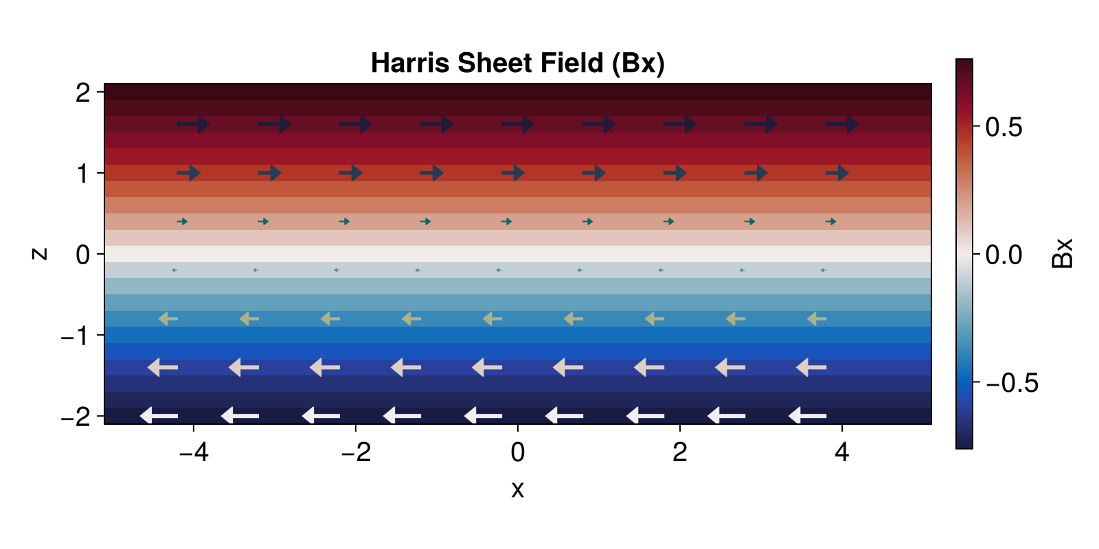

Asymmetric Harris Sheet

An asymmetric version of the Harris sheet where the magnetic field strength on either side can be different.

$$B_x(z)=\frac{B_1+B_2}{2}+\frac{B_1-B_2}{2}\tanh \left(\frac{z}{L}\right)$$

B1, B2, L = 2.0, 1.0, 2.0
sheet_asym = AsymmetricHarrisSheet(B1, B2, L)

zs = range(-5, 5, length=100)
Bxs = [sheet_asym(SVector(0.0, 0.0, z))[1] for z in zs]

fig = Figure()
ax = Axis(fig[1, 1], xlabel="z", ylabel="Bx", title="Asymmetric Harris Sheet Profile")
lines!(ax, zs, Bxs)
fig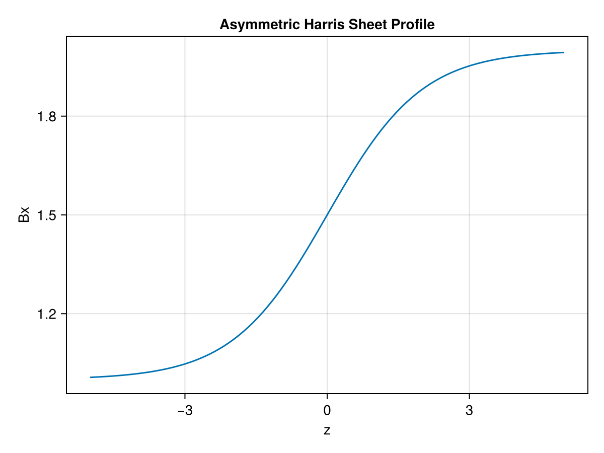

Force-Free Harris Sheet

A force-free current sheet configuration where the magnetic pressure is constant.

$$\begin{array}{rl}{B}_x(z)& =B_0\tanh (z/L)\\ B_y(z)& =B_0\mathrm{sech}(z/L)\end{array}$$

B0, L = 1.0, 2.0
sheet_ff = ForceFreeHarrisSheet(B0, L)

zs = range(-5, 5, length=100)
Bxs = [sheet_ff(SVector(0.0, 0.0, z))[1] for z in zs]
Bys = [sheet_ff(SVector(0.0, 0.0, z))[2] for z in zs]
Bzs =  @. sqrt(Bxs^2 + Bys^2)

fig = Figure()
ax = Axis(fig[1, 1], xlabel="z", ylabel="B", title="Force-Free Harris Sheet")
lines!(ax, zs, Bxs, label="Bx")
lines!(ax, zs, Bys, label="By")
lines!(ax, zs, Bzs, label="|B|", linestyle=:dash)
axislegend(ax)
fig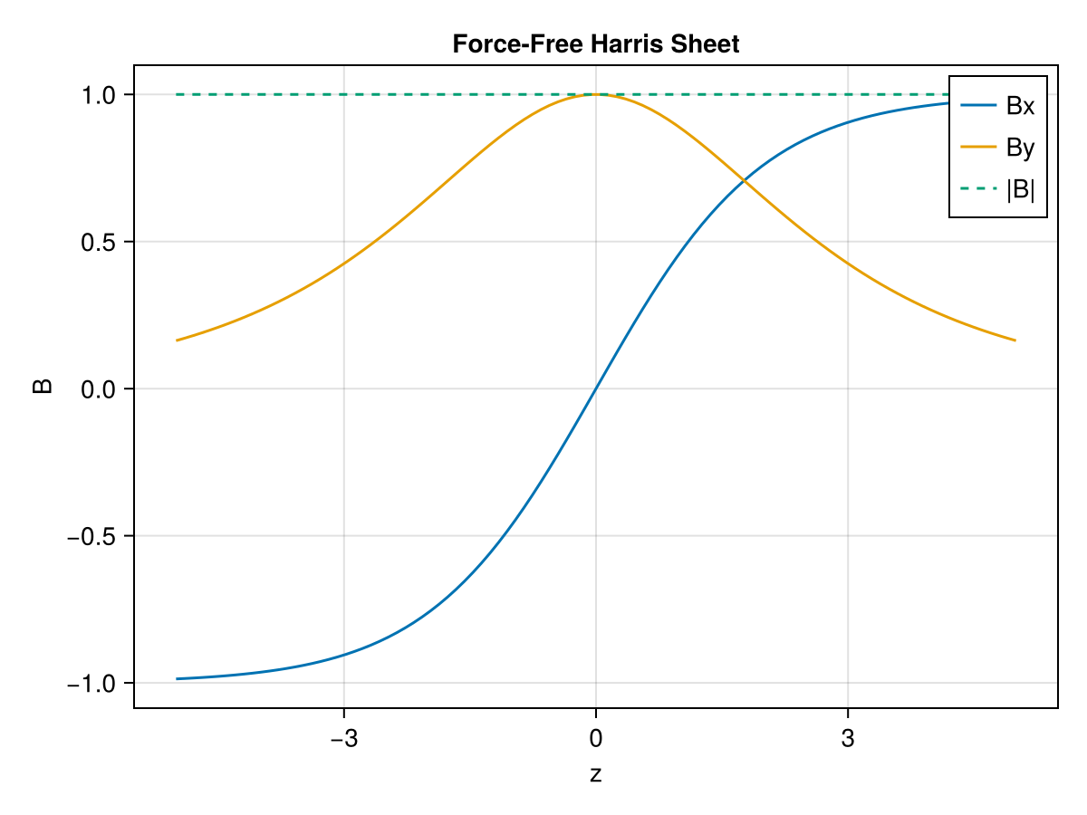

Bifurcated Harris Sheet

A current sheet model with two peaks in the current density, often observed in the Earth's magnetotail.

$$B_x(z)=\frac{B_0}{2}[\tanh \left(\frac{z-d}{L}\right)+\tanh \left(\frac{z+d}{L}\right)]$$

B0, L, d = 1.0, 2.0, 1.5
sheet_bif = BifurcatedHarrisSheet(B0, L, d)

zs = range(-10, 10, length=200)
Bxs = [sheet_bif(SVector(0.0, 0.0, z))[1] for z in zs]

fig = Figure()
ax = Axis(fig[1, 1], xlabel="z", ylabel="Bx", title="Bifurcated Harris Sheet Profile")
lines!(ax, zs, Bxs)
fig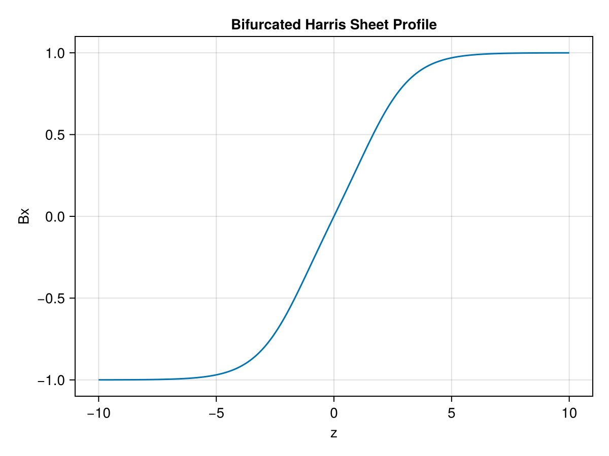

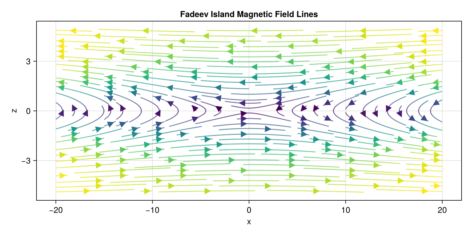
Fadeev Island

The Fadeev island model describes a chain of magnetic islands (magnetic reconnection).

$$A_y(x,z)=-B_{0}L\ln [\cosh (z/L)+ϵ\cos (x/L_x)]$$

B0, L, Lx, ε = 1.0, 2.0, 10.0, 0.5
fadeev = FadeevIsland(B0, L, Lx, ε)

xs = range(-20, 20, length=100)
zs = range(-5, 5, length=50)

# Calculate B components for streamplot
# Bx = -B0 * sinh(z/L) / denom
# Bz = -B0 * L * ε * sin(x/Lx) / Lx / denom

fig = Figure(size=(800, 400))
ax = Axis(fig[1, 1], xlabel="x", ylabel="z", title="Fadeev Island Magnetic Field Lines")

# Streamplot to visualize the islands
streamplot!(ax, (x, z) -> Point2f(fadeev(SVector(x, 0, z))[1], fadeev(SVector(x, 0, z))[3]),
    -20..20, -5..5, colormap=:viridis)
fig