Biot-Savart Solver

The magnetic field for a finite wire segment is calculated using the algebraic form of the Biot-Savart law:

$$\mathbf{B}=\frac{{\mu }_{0}I}{4\pi }\frac{d\mathbf{l}\times \mathbf{a}}{|d\mathbf{l}\times \mathbf{a}{|}^2}(\frac{d\mathbf{l}\cdot \mathbf{a}}{|\mathbf{a}|}-\frac{d\mathbf{l}\cdot \mathbf{b}}{|\mathbf{b}|})$$

where $\mathbf{a}=\mathbf{r}-{\mathbf{r}}_{start}$ and $\mathbf{b}=\mathbf{r}-{\mathbf{r}}_{end}$ are vectors from the ends of the segment to the observation point $\mathbf{r}$, and $d\mathbf{l}={\mathbf{r}}_{end}-{\mathbf{r}}_{start}$ is the segment vector.

For arbitrary wire geometries, discretize the path and sum the contributions.

using Magnetostatics, StaticArrays, LinearAlgebra
using CairoMakie

# Define a circular loop and discretize it
loop = CurrentLoop(1.0, 1.0, [0, 0, 0], [0, 0, 1])
wire = discretize_loop(loop, 100)

# Define the solver
solver = BiotSavart()

# Solve for B at a point
r = SVector(0.0, 0.0, 0.5)
B = solve(solver, wire, r)
println("B at $r: $B [T]")

B at [0.0, 0.0, 0.5]: [-1.4475660719677984e-23, 1.3609706015911533e-23, 4.4964729452166677e-7] [T]

Visualizing the result:

xs = range(-2, 2, length=51)
zs = range(-2, 2, length=51)

function field_xz_bs(x, z)
    B = solve(solver, wire, SVector(x, 0.0, z))
    return Point2f(B[1], B[3])
end

fig = Figure(size = (700, 600), fontsize=20)
ax = Axis(fig[1, 1];
    xlabel="x", ylabel="z", aspect=DataAspect(), title="Biot-Savart Loop Field")

Bmag = [norm(solve(solver, wire, SVector(x, 0.0, z))) for x in xs, z in zs]
hm = heatmap!(ax, xs, zs, log10.(Bmag .+ 1e-9), colormap=:plasma)
Colorbar(fig[1, 2], hm, label="log10(|B|)")

streamplot!(ax, field_xz_bs, -2..2, -2..2;
    arrow_size = 8, linewidth = 1.5)

fig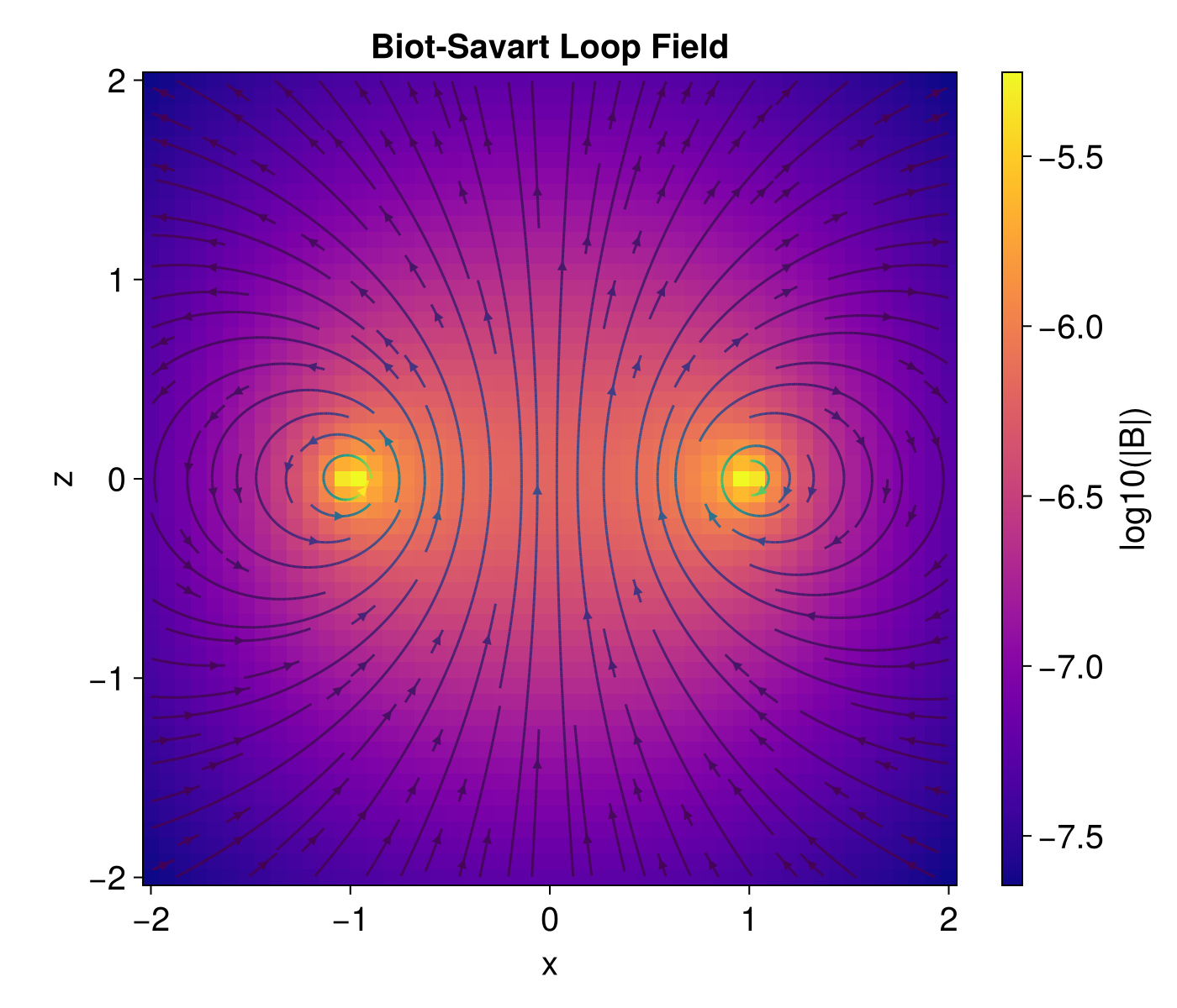

Conducting Wall (Method of Images)

A perfectly-conducting plane forces the normal component of $\mathbf{B}$ to zero at its surface. For a long straight wire carrying current $I$ at height $h$ above a conducting plane, the solution is given exactly by the method of images: an image wire at $-h$ carries the opposite current $-I$, so their combined normal (perpendicular-to-wall) components cancel at $z=0$.

using Magnetostatics, StaticArrays, LinearAlgebra

# Wire along the y-axis at height h above the wall z = 0
h     = 1.0   # height above the wall [m]
I_w   = 1.0   # current [A]
L     = 10.0  # half-length of the wire approximating an infinite wire

wire_wall = Wire(
    [SVector(0.0, -L, h), SVector(0.0, L, h)],
    I_w
)

bc_wall   = ConductingWall(3, 0.0)   # wall normal along z-axis (axis=3), at z=0
solver_wall = BiotSavart(bc_wall)

B_wall(x, z) = solve(solver_wall, wire_wall, SVector(x, 0.0, z))

# Visualise field in the xz half-plane above the wall
xs_w = range(-4.0, 4.0, length=61)
zs_w = range(0.0,  4.0, length=31)

Bmag_w = [norm(B_wall(x, z)) for x in xs_w, z in zs_w]

fig_wall = Figure(size=(700, 500), fontsize=20)
ax_wall  = Axis(fig_wall[1, 1];
    xlabel="x [m]", ylabel="z [m]", aspect=DataAspect(),
    title="Wire above Conducting Wall (z = 0)")

hm_w = heatmap!(ax_wall, xs_w, zs_w, log10.(Bmag_w .+ 1e-9); colormap=:plasma)
Colorbar(fig_wall[1, 2], hm_w; label="log10(|B| / T)")

streamplot!(ax_wall,
    (x, z) -> let B = B_wall(Float64(x), Float64(z)); Point2f(B[1], B[3]) end,
    -4..4, 0..4; arrow_size=8, linewidth=1.5)

# Wall boundary
hlines!(ax_wall, [0.0]; color=:white, linewidth=2, linestyle=:dash)
scatter!(ax_wall, [0.0], [h]; color=:yellow, markersize=12, label="wire")
axislegend(ax_wall; position=:rt)

fig_wall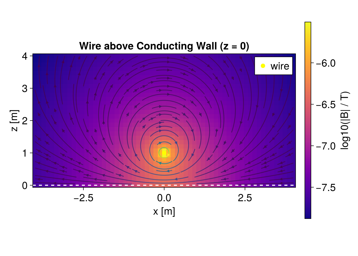

Analytical verification

At the wall surface ($z=0$), $B_z$ must vanish by the boundary condition. The on-wall $B_z$ from the real wire and its image along the x-direction is:

$$B_z(x,0)=\frac{{\mu }_{0}I}{2\pi }\frac{h}{x^2+h^2}-\frac{{\mu }_{0}I}{2\pi }\frac{h}{x^2+h^2}=0$$

and can be verified numerically:

xs_check = range(-4.0, 4.0, length=40)
Bz_at_wall = [B_wall(x, 1e-6)[3] for x in xs_check]   # just above z=0
println("max |Bz| at wall: ", maximum(abs, Bz_at_wall))

max |Bz| at wall: 2.571778923433936e-13

Conducting Sphere in a Uniform Background Field

A perfectly-conducting sphere expels all magnetic flux from its interior. When placed in an external field ${\mathbf{B}}_0=B_0\hat{z}$, the sphere develops induced surface currents $\mathbf{K}$ whose field exactly cancels the normal component of ${\mathbf{B}}_0$ on the sphere surface. Outside the sphere, the total field is the superposition of ${\mathbf{B}}_0$ and the field of a magnetic dipole whose moment is chosen to cancel $\mathbf{B}\cdot \hat{r}$ at $r=R$:

$${\mathbf{B}}_{\mathrm{out}}=B_0\hat{z}+\frac{{\mu }_0}{4\pi }\frac{3(\mathbf{m}\cdot \hat{r})\hat{r}-\mathbf{m}}{r^3},\mathbf{m}=-\frac{2\pi }{{\mu }_0}{B}_0{R}^3\hat{z}$$

The negative sign on $\mathbf{m}$ means the image dipole opposes the background field. Here we approximate the uniform background with a Helmholtz coil pair (two large co-axial loops of equal current separated by one loop radius), then use the ConductingSphere BEM solver to find the induced surface currents numerically.

using Magnetostatics, StaticArrays, LinearAlgebra

# --- Problem parameters ---
B0 = 1.0   # background field magnitude [T]
R  = 1.0   # sphere radius [m]

# Approximate B0 ẑ with a Helmholtz pair (radius 10R, separation 10R)
# Each loop current chosen so that B_z at the origin equals B0.
# For a Helmholtz pair: B_z = μ0 I R² / (R²+(R/2)²)^(3/2) (two loops)
R_coil  = 10R
I_coil  = B0 * (R_coil^2 + (R_coil/2)^2)^(3/2) / (Magnetostatics.μ₀ * R_coil^2)
loop_p  = discretize_loop(R_coil, 200, I_coil;
              center=SVector(0.0, 0.0,  R_coil/2), normal=SVector(0.0, 0.0, 1.0))
loop_m  = discretize_loop(R_coil, 200, I_coil;
              center=SVector(0.0, 0.0, -R_coil/2), normal=SVector(0.0, 0.0, 1.0))

# Combine into a single Wire for the BEM (concatenate segments)
helmholtz = Wire(
    vcat(loop_p.points, loop_m.points),
    I_coil
)

# --- BEM solve for the conducting sphere ---
bc   = ConductingSphere(SVector(0.0, 0.0, 0.0), R, 32, 64)
mesh = compute_surface_current(bc, helmholtz)

bare = BiotSavart()
B_total(r) = solve(bare, helmholtz, r) + solve(bare, mesh, r)

# --- Visualisation: field lines in the xz-plane ---
xs = range(-3R, 3R, length=61)
zs = range(-3R, 3R, length=61)

# Mask points inside the sphere (field is zero there)
in_sphere(x, z) = sqrt(x^2 + z^2) < R

fig2 = Figure(size=(700, 650), fontsize=20)
ax2  = Axis(fig2[1, 1];
    xlabel="x / R", ylabel="z / R", aspect=DataAspect(),
    title="Conducting Sphere (R=1) in Uniform Bz")

Bmag = [in_sphere(x, z) ? NaN :
        norm(B_total(SVector(x, 0.0, z))) for x in xs, z in zs]
hm = heatmap!(ax2, xs ./ R, zs ./ R, log10.(Bmag .+ 1e-9); colormap=:plasma)
Colorbar(fig2[1, 2], hm; label="log10(|B| / T)")

streamplot!(ax2,
    (x, z) -> in_sphere(x, z) ?
        Point2f(0, 0) :
        let B = B_total(SVector(Float64(x*R), 0.0, Float64(z*R)))
            Point2f(B[1], B[3])
        end,
    -3..3, -3..3; arrow_size=8, linewidth=1.5)

# Draw sphere boundary
θs = range(0, 2π, length=200)
lines!(ax2, cos.(θs), sin.(θs); color=:white, linewidth=2, linestyle=:dash)

fig2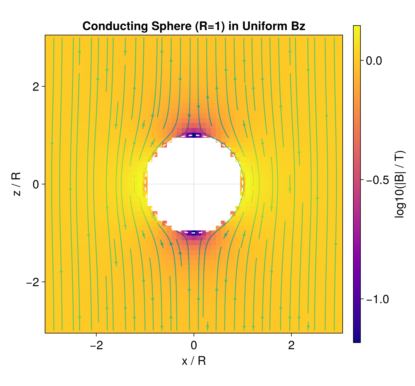

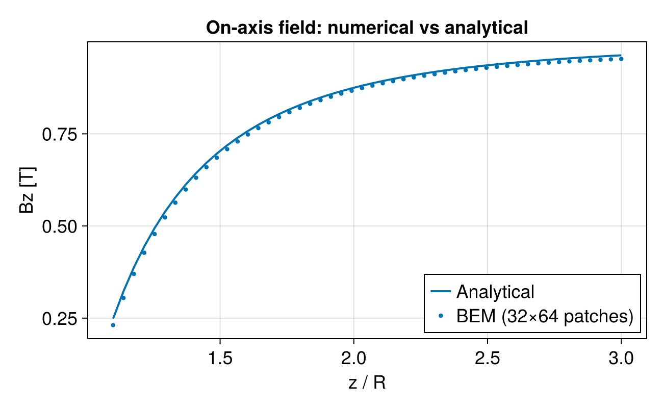
Analytical validation

On the positive z-axis at $r>R$, the total field has only a z-component. The image dipole cancels exactly half the background at $r=R$, giving zero normal flux there:

$$B_z(0,0,z)=B_0(1-\frac{R^3}{z^3})$$

At $z=R$ this is zero; as $z\to \mathrm{\infty }$ it recovers $B_0$.

zs_axis = range(1.1R, 3R, length=50)
Bz_num  = [B_total(SVector(0.0, 0.0, z))[3] for z in zs_axis]
Bz_ana  = @. B0 * (1 - R^3 / zs_axis^3)

fig3 = Figure(size=(650, 400), fontsize=18)
ax3  = Axis(fig3[1, 1];
    xlabel="z / R", ylabel="Bz [T]",
    title="On-axis field: numerical vs analytical")
lines!(ax3, zs_axis ./ R, Bz_ana; label="Analytical", linewidth=2)
scatter!(ax3, zs_axis ./ R, Bz_num; label="BEM (32×64 patches)", markersize=6)
axislegend(ax3; position=:rb)
fig3