Select and plot particles with flekspy

This example loads the small AMReX particle fixture used by the documentation, projects particle velocities into a field-aligned frame, selects particles inside a velocity-space region, and plots the resulting distributions.

The fixture is downloaded from the same source as amrex_data.ipynb. The notebook downloads it at runtime, so generated data and plot outputs do not need to be stored in the repository.

from pathlib import Path

import flekspy
import matplotlib.pyplot as plt
import numpy as np

from flekspy.util import download_testfile

download_testfile(
    "https://raw.githubusercontent.com/henry2004y/batsrus_data/master/3d_particle.tar.gz",
    "data",
)
data_file = Path("data/3d_particle_region0_1_t00000002_n00000007_amrex")
ds = flekspy.load(str(data_file), use_yt_loader=True)
print(f"Loaded {data_file}")

yt : [INFO     ] 2026-09-18 03:21:34,980 Parameters: current_time              = 2.066624095642792

yt : [INFO     ] 2026-09-18 03:21:34,984 Parameters: domain_dimensions         = [64 40  1]

yt : [INFO     ] 2026-09-18 03:21:34,984 Parameters: domain_left_edge          = [-0.016 -0.01   0.   ]

yt : [INFO     ] 2026-09-18 03:21:34,985 Parameters: domain_right_edge         = [0.016 0.01  1.   ]

Loaded data/3d_particle_region0_1_t00000002_n00000007_amrex

The documented fixture is two-dimensional in position. We use the magnetic field components from the mesh to define a simple field-aligned frame and subtract the mean particle velocity before projecting.

data = ds.all_data()

x = np.asarray(data["particles", "p_x"])
y = np.asarray(data["particles", "p_y"])
ux = np.asarray(data["particles", "p_ux"])
uy = np.asarray(data["particles", "p_uy"])
uz = np.asarray(data["particles", "p_uz"])

bx = np.asarray(data["boxlib", "Bx"]).mean()
by = np.asarray(data["boxlib", "By"]).mean()
bz = np.asarray(data["boxlib", "Bz"]).mean()
b_vec = np.array([bx, by, bz])
if np.linalg.norm(b_vec) == 0:
    b_vec = np.array([0.0, 0.0, 1.0])
unit_b = b_vec / np.linalg.norm(b_vec)
reference = np.array([1.0, 0.0, 0.0])
unit_vb = np.cross(unit_b, reference)
if np.linalg.norm(unit_vb) == 0:
    reference = np.array([0.0, 1.0, 0.0])
    unit_vb = np.cross(unit_b, reference)
unit_vb /= np.linalg.norm(unit_vb)

velocity = np.column_stack((ux, uy, uz))
velocity -= velocity.mean(axis=0)
vel_b = velocity @ unit_b
vel_vb = velocity @ unit_vb
print(f"Selected fixture contains {len(x):,} particles")

Selected fixture contains 256,423 particles

Velocity distribution and particle selection

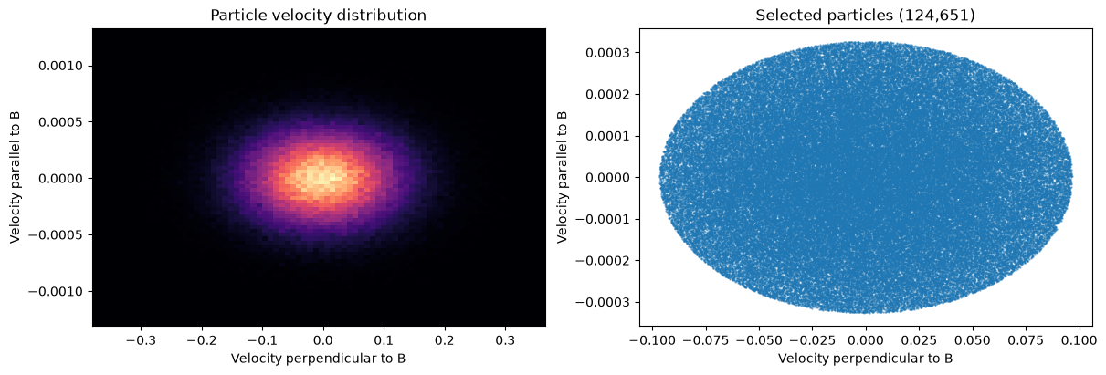
The first plot is a velocity distribution function in the two projected directions. The ellipse selects a lower-energy subset for subsequent analysis.

fig, axes = plt.subplots(1, 2, figsize=(12, 4), constrained_layout=True)
axes[0].hist2d(vel_vb, vel_b, bins=80, cmap="magma")
axes[0].set_xlabel("Velocity perpendicular to B")
axes[0].set_ylabel("Velocity parallel to B")
axes[0].set_title("Particle velocity distribution")

scale_vb = np.percentile(np.abs(vel_vb), 75)
scale_b = np.percentile(np.abs(vel_b), 75)
inside = (vel_vb / scale_vb) ** 2 + (vel_b / scale_b) ** 2 <= 1
axes[1].scatter(vel_vb[inside], vel_b[inside], s=0.5, alpha=0.5)
axes[1].set_xlabel("Velocity perpendicular to B")
axes[1].set_ylabel("Velocity parallel to B")
axes[1].set_title(f"Selected particles ({inside.sum():,})")
plt.show()

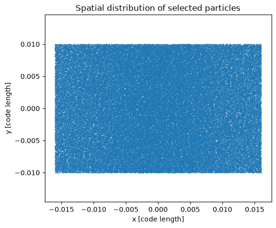
Spatial distribution of the selected particles

plt.figure(figsize=(6, 5))
plt.scatter(x[inside], y[inside], s=0.5, alpha=0.5)
plt.xlabel("x [code length]")
plt.ylabel("y [code length]")
plt.title("Spatial distribution of selected particles")
plt.axis("equal")
plt.show()