FLEKS Python Visualization Toolkit: Test Particle Data

flekspy is a Python package for processing FLEKS data. This notebook focuses on handling test particle data.

FLEKS data format

• Field: *.out format or AMREX built-in format, whose directory name is assumed to end with “_amrex”

• PIC particle: AMREX built-in format

• Test particle: binary data format

Importing the package

import flekspy

Downloading demo data

Example test particle data can be downloaded as follows:

from flekspy.util import download_testfile

url = "https://raw.githubusercontent.com/henry2004y/batsrus_data/master/test_particles_PBEG.tar.gz"
download_testfile(url, "data")

Plotting Test Particle Trajectories

Loading particle data

from flekspy import FLEKSTP

tp = FLEKSTP("data/test_particles_PBEG", iSpecies=1)

Obtaining particle IDs

Test particle IDs consists of a CPU index and a particle index attached to the CPU.

tp.getIDs()

[(0, 3), (0, 4)]

Reading particle trajectory

tp[0].collect()

shape: (5, 22)

time	x	y	z	vx	vy	vz	bx	by	bz	ex	ey	ez	dbxdx	dbxdy	dbxdz	dbydx	dbydy	dbydz	dbzdx	dbzdy	dbzdz
f32	f32	f32	f32	f32	f32	f32	f32	f32	f32	f32	f32	f32	f32	f32	f32	f32	f32	f32	f32	f32	f32
0.0	0.000128	-0.000795	0.0	0.000042	0.000067	0.000016	224199.65625	281.65274	11182.642578	-0.447306	3.064687	8.890797	0.0	0.0	0.0	2.1949e6	0.0	0.0	-107828.21875	0.0	0.0
0.286543	0.000134	-0.000786	0.000002	0.000042	0.000068	0.000014	224414.28125	207.771286	11134.431641	-1.991942	3.305334	8.97459	-225897.34375	123607.867188	0.0	1.993212e6	110127.578125	0.0	-52048.246094	458591.0	0.0
0.573086	0.000146	-0.000766	0.000002	0.000042	0.000069	0.000012	224547.4375	171.823151	11111.666016	-1.018998	2.346379	8.844476	-159384.8125	358307.84375	0.0	2.0199e6	25620.753906	0.0	68019.898438	1.3220e6	0.0
0.864857	0.000159	-0.000745	0.000002	0.000042	0.000071	0.000011	224356.78125	25.654217	11075.149414	1.378713	3.30056	9.281602	385832.53125	685539.1875	0.0	2.0586e6	-450143.34375	0.0	668866.25	693783.875	0.0
1.157084	0.000171	-0.000724	0.000001	0.000043	0.000072	0.000009	224224.421875	-133.657379	10893.328125	0.683855	2.13601	9.826899	822001.0	1.3780e6	0.0	1.7280e6	-886848.8125	0.0	1.0217e6	-653294.8125	0.0

Getting initial location

x = tp.read_initial_condition(tp.getIDs()[0])
print("time, X, Y, Z, Vx, Vy, Vz")
print(
    f"{x[0]:.2e}, {x[1]:.2e}, {x[2]:.2e}, {x[3]:.2e}, {x[4]:.2e}, {x[5]:.2e}, {x[6]:.2e}"
)

time, X, Y, Z, Vx, Vy, Vz
0.00e+00, 1.28e-04, -7.95e-04, 0.00e+00, 4.21e-05, 6.65e-05, 1.55e-05

Interpolate particles trajectory at selected times

from flekspy.tp import interpolate_at_times

interpolate_at_times(tp[0], [1.0])

shape: (1, 22)

time	x	y	z	vx	vy	vz	bx	by	bz	ex	ey	ez	dbxdx	dbxdy	dbxdz	dbydx	dbydy	dbydz	dbzdx	dbzdy	dbzdz
f32	f32	f32	f32	f32	f32	f32	f32	f32	f32	f32	f32	f32	f32	f32	f32	f32	f32	f32	f32	f32	f32
1.0	0.000165	-0.000736	0.000001	0.000042	0.000071	0.00001	224295.5625	-48.021412	10991.063477	1.057367	2.761999	9.533781	587544.0625	1.0058e6	0.0	1.90571e6	-652103.1875	0.0	832021.6875	70810.625	0.0

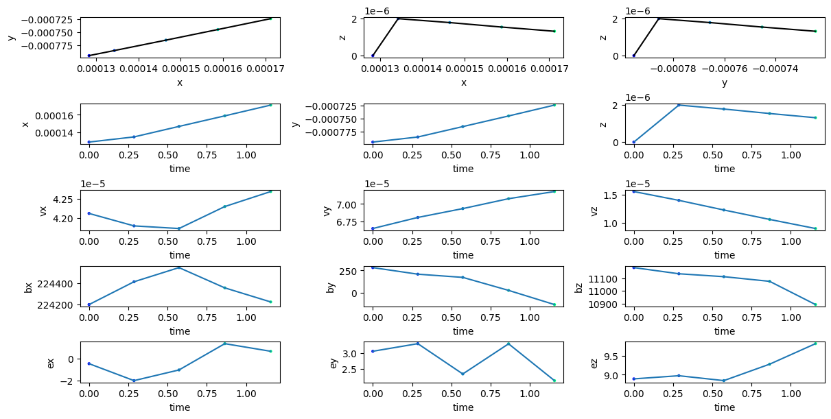
Plotting trajectory

import matplotlib.pyplot as plt
tp.plot_trajectory(tp.getIDs()[0])
plt.show()

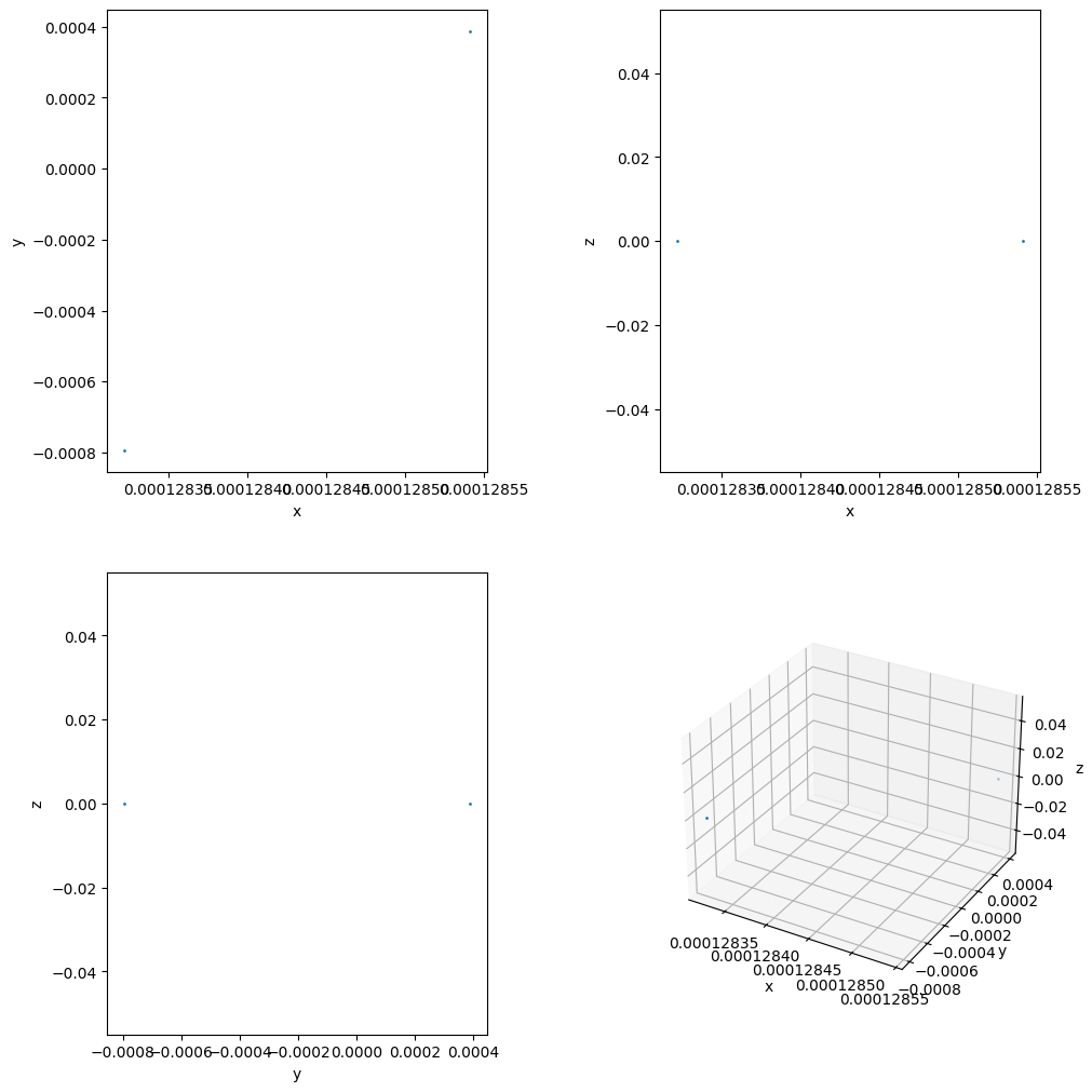
Reading and visualizing all particle’s location at a given snapshot

ids, pData = tp.read_particles_at_time(0.0, doSave=False)
tp.plot_location(pData)
plt.show()

Selecting particles starting in a region

from flekspy.tp import Indices

def f_select(tp, pid):
    pData = tp.read_initial_condition(pid)
    inRegion = pData[Indices.X] > 0 and pData[Indices.Y] > 0
    return inRegion


pSelected = tp.select_particles(f_select)

Saving trajectories to CSV

tp.save_trajectory_to_csv(tp.getIDs()[0])

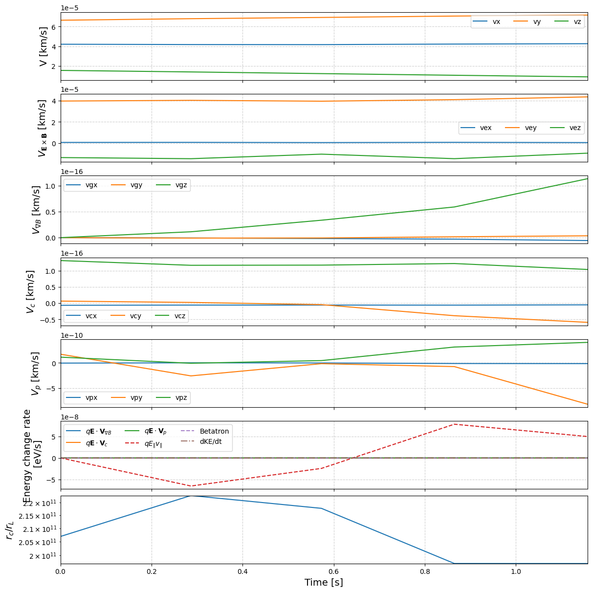
Calculating drifts

With the $\mathbf{E}, \mathbf{B}$, and $\nabla \mathbf{B}$ saved along the trajectory, we can compute various drifts:

• Convection drift velocity: tp.get_ExB_drift(pid)

• Curvature drift velocity: tp.get_curvature_drift(pid)

• Gradient drift velocity: tp.get_gradient_drift(pid)

• Polarization drift velocity: tp.get_polarization_drift(pid)

The first adiabatic assumption can be checked by comparing the ratio between the curvature length and the gyroradius $r_c / r_L$ via get_adiabaticity_parameter. If $r_c / r_L \gg 1$, then the gyromotion can be savely ignored.

The Betatron acceleration $\mu \partial B/\partial t$ can be indirectly computed with the knowledge of total derivative $\mathrm{d}B/\mathrm{d}t$ and $\mathbf{v}\nabla B$ along the trajectory:

pid = tp.getIDs()[0]
pt = tp[pid]
mu = tp.get_first_adiabatic_invariant(pt)
pt = tp.get_betatron_acceleration(pt, mu)

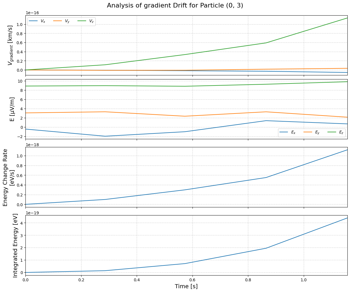
To analyze a specific drift:

tp.analyze_drift(pid, "gradient")

By combining all these together, we come up with time series of various terms:

tp.analyze_drifts(pid)

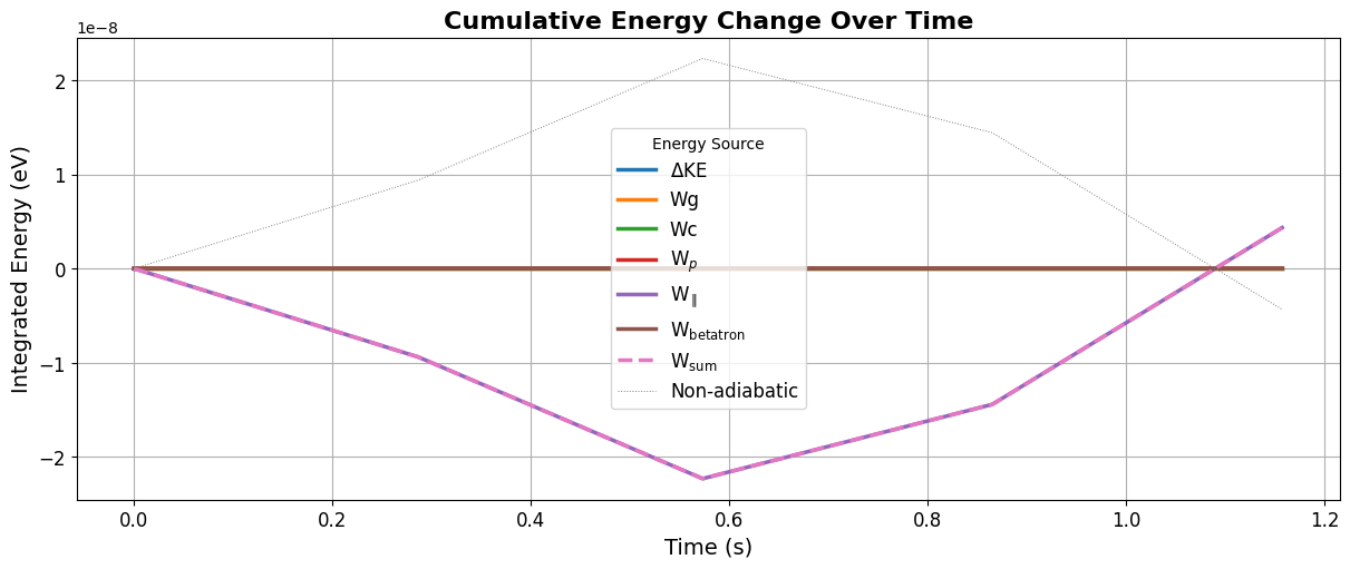
We can the track the energy change from drift and EM field variations:

from flekspy.tp import plot_integrated_energy

df = tp.integrate_drift_accelerations(tp.getIDs()[0])
plot_integrated_energy(df)

Alternatively, the energy change can be decomposed into three terms: the parallel acceleration, Betatron acceleration, and the Fermi acceleration:

df = tp.get_energy_change_guiding_center(tp.getIDs()[0])

df

shape: (5, 5)

time	dW_parallel	dW_betatron	dW_fermi	dW_total
f32	f32	f32	f32	f32
0.0	-1.2793e-15	7.9045e-14	1.1878e-18	7.7767e-14
0.286543	-6.5532e-8	6.6485e-14	1.0648e-18	-6.5532e-8
0.573086	-2.4509e-8	-1.0753e-14	1.0303e-18	-2.4509e-8
0.864857	7.8494e-8	-6.7355e-14	9.9597e-19	7.8494e-8
1.157084	4.9847e-8	-5.8379e-14	8.8976e-19	4.9847e-8