Exosphere Module

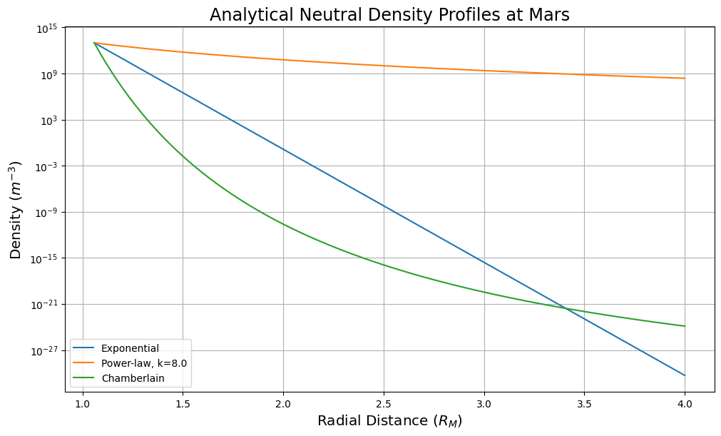
This notebook demonstrates the usage of the flekspy.util.exosphere module. We will use Mars as an example and plot three types of neutral density profiles: exponential, power-law, and Chamberlain.

import numpy as np
import matplotlib.pyplot as plt
from flekspy.util.exosphere import Exosphere

Mars Example

# Mars parameters
R_planet = 3390e3  # Mars radius [m]
M_planet = 6.42e23  # Mars mass [kg]
T_exo = 200  # Exospheric temperature [K]
H0 = 100e3 # Scale height [m]
n0 = 1e13  # Density at the exobase [m^-3]
m_neutral = 16 * 1.67e-27  # Mass of neutral oxygen [kg]
r0 = R_planet + 200e3 # Exobase radius [m]
k0 = 8.0 # Power-law exponents

mars_exo_exp = Exosphere(
    neutral_profile="exponential",
    n0=n0,
    H0=H0,
    T0=T_exo,
    exobase_radius=r0,
    M_planet=M_planet,
    m_neutral=m_neutral,
)
mars_exo_power = Exosphere(
    neutral_profile="power_law",
    n0=n0,
    H0=H0,
    T0=T_exo,
    k0=k0,
    exobase_radius=r0,
    M_planet=M_planet,
    m_neutral=m_neutral,
)
mars_exo_chamb = Exosphere(
    neutral_profile="chamberlain",
    n0=n0,
    H0=H0,
    T0=T_exo,
    exobase_radius=r0,
    M_planet=M_planet,
    m_neutral=m_neutral,
)

r = np.linspace(r0, 4 * R_planet, 100)
n_exp = mars_exo_exp.get_neutral_density(r)
n_power = mars_exo_power.get_neutral_density(r)
n_chamb = mars_exo_chamb.get_neutral_density(r)

plt.figure(figsize=(10, 6), constrained_layout=True)
plt.plot(r / R_planet, n_exp, label="Exponential")
plt.plot(r / R_planet, n_power, label=f"Power-law, k={k0}")
plt.plot(r / R_planet, n_chamb, label="Chamberlain")
plt.yscale("log")
plt.xlabel("Radial Distance ($R_M$)", fontsize="x-large")
plt.ylabel("Density ($m^{-3}$)", fontsize="x-large")
plt.title("Analytical Neutral Density Profiles at Mars", fontsize="xx-large")
plt.legend()
plt.grid(True)
plt.show()