Magnetic Reconnection Analysis with flekspy

This notebook demonstrates how to analyze magnetic reconnection simulations using flekspy.

Capabilities covered:

1. Vector Potential \(A_z(x, y)\): Conservative 2D path integration from the central column outward such that \(\mathbf{B} = \nabla \times (A_z \hat{\mathbf{z}})\).

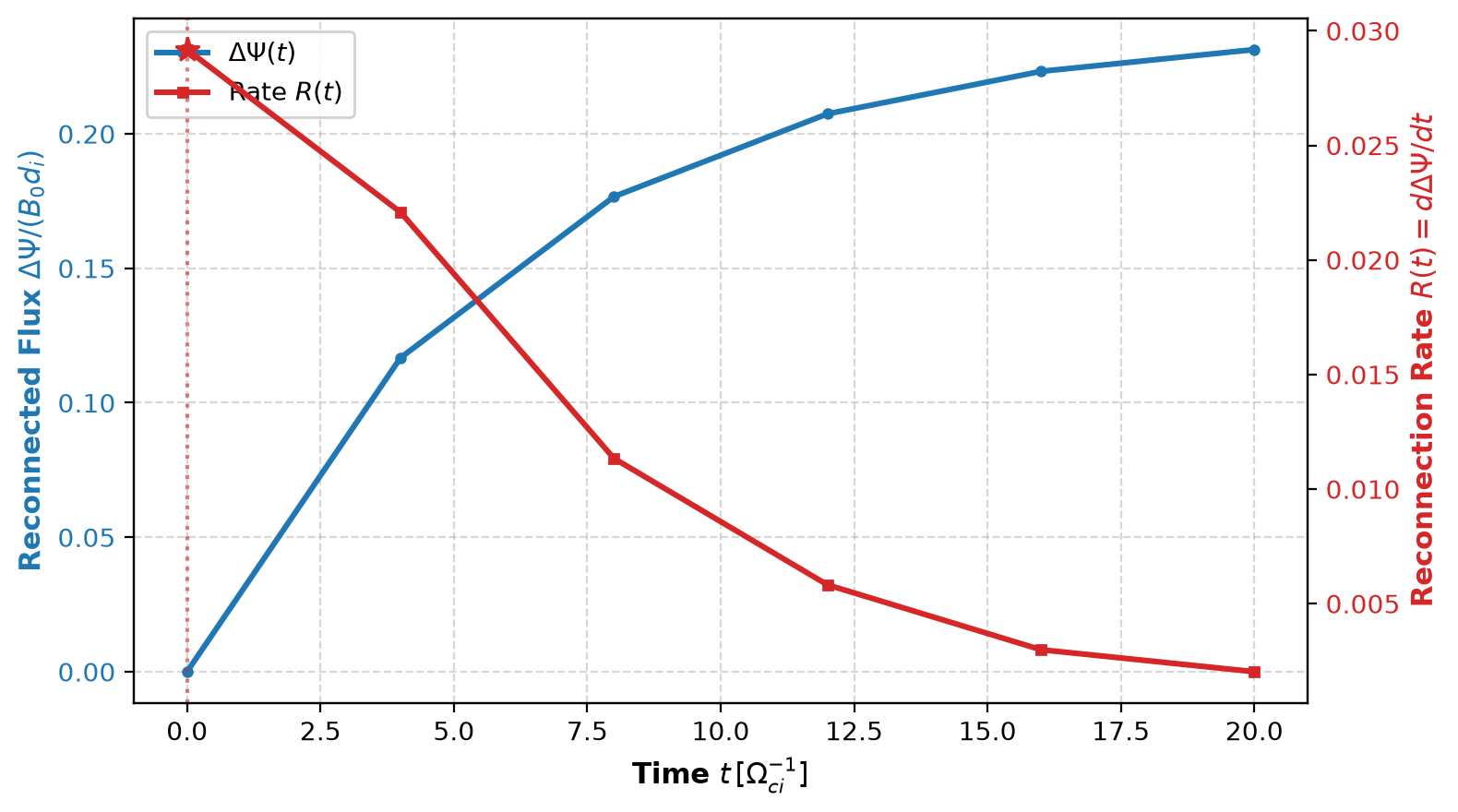
2. Reconnected Flux \(\Delta\Psi(t)\) & Reconnection Rate \(R(t)\): Evaluated from midplane magnetic flux or vector potential.

3. ReconnectionSeries Container: Fast header scanning, lazy loading with LRU cache, and single-pass metrics extraction for time series.

4. xarray Dataset Accessor: Seamless integration via ds.reconnection.

5. Publication-Grade Visualizations: Continuous magnetic field streamlines with directional arrows via flekspy.plot.streamplot.

Full-scale kinetic or Hall-MHD reconnection runs typically produce gigabytes of output. In this notebook, we generate a compact sequence of synthetic snapshots to showcase the complete analysis workflow without requiring external downloads.

1. Imports and Setup

import tempfile
from pathlib import Path
import matplotlib.pyplot as plt
import numpy as np
import xarray as xr

import flekspy as fs
import flekspy.reconnection as reconn

# Configure display options
xr.set_options(display_expand_coords=False, display_expand_data=False)
plt.rcParams["figure.dpi"] = 120

2. Generating Synthetic Reconnection Snapshots

We construct a sequence of snapshots simulating the physical stages of magnetic reconnection:

• An initial Harris current sheet: \(B_x(y) = B_0 \tanh(y/L)\)

• An island perturbation that grows over time: \(b_1(t)\)

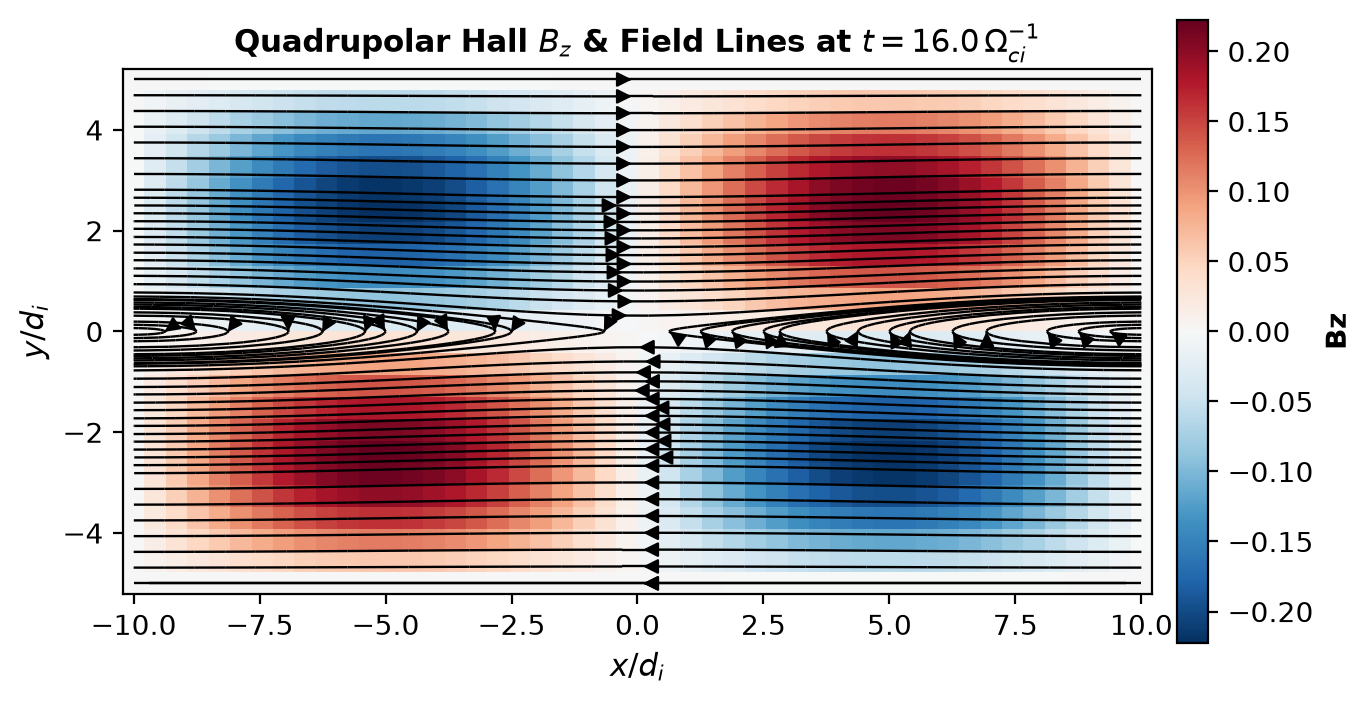
• The characteristic out-of-plane quadrupolar Hall magnetic field \(B_z(x, y)\)

• Bipolar reconnection outflow jets \(u_x(x, y)\)

Each snapshot is saved as a standard IDL ASCII output file (.out).

temp_dir = tempfile.TemporaryDirectory()
data_dir = Path(temp_dir.name)

nx, ny = 48, 24
Lx, Ly = 20.0, 10.0
x = np.linspace(-Lx / 2, Lx / 2, nx)
y = np.linspace(-Ly / 2, Ly / 2, ny)

# Generate 6 time snapshots showing island growth
times = [0.0, 4.0, 8.0, 12.0, 16.0, 20.0]
file_paths = []

for i, t in enumerate(times):
    # Reconnection perturbation amplitude grows and then saturates
    amp = 0.12 * (1.0 - np.exp(-t / 6.0))
    fpath = data_dir / f"z=0_var_t{t:05.1f}_n{i*200:04d}.out"
    
    lines = [
        "PIC unit",
        f"{i * 200} {t:.4f} 2 0 6",
        f"{nx} {ny}",
        "x y Bx By Bz ux"
    ]
    
    for j_idx in range(ny):
        for i_idx in range(nx):
            xi = x[i_idx]
            yj = y[j_idx]
            bx_val = np.tanh(yj) - amp * (np.pi / Ly) * np.cos(2 * np.pi * xi / Lx) * np.sin(np.pi * yj / Ly)
            by_val = amp * (2 * np.pi / Lx) * np.sin(2 * np.pi * xi / Lx) * np.cos(np.pi * yj / Ly)
            bz_val = 0.25 * amp * 8.0 * np.sin(2 * np.pi * xi / Lx) * np.sin(2 * np.pi * yj / Ly)
            ux_val = 0.5 * (amp / 0.12) * np.sin(2 * np.pi * xi / Lx) * np.exp(-(yj / 1.5)**2)
            lines.append(f"{xi:.5e} {yj:.5e} {bx_val:.5e} {by_val:.5e} {bz_val:.5e} {ux_val:.5e}")
            
    fpath.write_text("\n".join(lines) + "\n")
    file_paths.append(str(fpath))

print(f"Generated {len(file_paths)} synthetic snapshots in {data_dir}")

Generated 6 synthetic snapshots in /tmp/tmp74b6xxah

3. Single-Snapshot Analysis and Xarray Accessor

flekspy registers an xarray accessor ds.reconnection on every 2D dataset loaded with read_idl or load.

Let’s load the snapshot near peak reconnection (\(t = 16.0\)) and inspect the accessor capabilities:

ds_peak = fs.read_idl(file_paths[4])
print(f"Loaded frame at t = {ds_peak.attrs['time']:.1f} with dimensions: {dict(ds_peak.sizes)}")

# 1. Calculate 2D magnetic vector potential Az(x, y)
az = ds_peak.reconnection.calc_vector_potential()
print(f"Vector potential Az computed: shape = {az.shape}, range = [{az.min().item():.3f}, {az.max().item():.3f}]")

# 2. Calculate reconnected magnetic flux Delta Psi
flux_mid = ds_peak.reconnection.reconnected_flux(method="midplane")
flux_az = ds_peak.reconnection.reconnected_flux(method="az")
print(f"Reconnected flux (midplane integral): {flux_mid:.4f}")
print(f"Reconnected flux (vector potential):  {flux_az:.4f}")

Loaded frame at t = 16.0 with dimensions: {'x': 48, 'y': 24}
Vector potential Az computed: shape = (48, 24), range = [-4.380, 0.000]
Reconnected flux (midplane integral): 0.2232
Reconnected flux (vector potential):  0.2222

2D Slice with Continuous Field Lines and Directional Arrows

plot_2d_slice combines the scalar background field (such as the Hall field \(B_z\) or outflow \(u_x\)) with continuous magnetic streamlines that include directional arrowheads:

fig, ax = ds_peak.reconnection.plot_slice(
    var="Bz",
    stream_field="B",
    stream_density=1.1,
    title=r"Quadrupolar Hall $B_z$ & Field Lines at $t = 16.0 \, \Omega_{ci}^{-1}$",
)
plt.show()

4. Multi-Frame Analysis with ReconnectionSeries

ReconnectionSeries inherits from IDLSeries, which provides fast header pre-scanning and lazy on-demand loading with an LRU cache (max_cache=32 by default).

It automatically extracts the time series of:

• Reconnected flux \(\Delta\Psi(t)\)

• Reconnection rate \(R(t) = d\Delta\Psi/dt\)

• Peak quadrupolar Hall field \(\max(|B_z|)\)

• Peak outflow velocity \(\max(|u_x|)\)

series = fs.ReconnectionSeries(f"{data_dir}/*.out", max_cache=4)
print(series)

# Summary dictionary
summary = series.summary()
print("\nReconnection Summary:")
for key, val in summary.items():
    print(f"  {key}: {val}")

<ReconnectionSeries: 6 frames, t=[0.00, 20.00], grid=[48 24], mode=lazy(lru=4), vars=[np.str_('x'), np.str_('y'), np.str_('Bx'), np.str_('By'), np.str_('Bz'), np.str_('ux')]>

Reconnection Summary:
  peak_rate: 0.02918110265957447
  peak_time: 0.0
  peak_frame: 0
  max_flux: 0.23132818936170213
  peak_hall_bz: 0.23077
  peak_outflow_ux: 0.471878
  total_frames: 6
  time_range: (0.0, 20.0)

5. Reconnection Rate vs Time

plot_reconnection_rate displays the reconnected flux \(\Delta\Psi(t)\) on the left axis and the reconnection rate \(R(t) = d\Delta\Psi/dt\) on the right axis, highlighting the peak reconnection rate:

fig, (ax1, ax2) = reconn.plot_reconnection_rate(series)
plt.show()

6. Multi-Panel Peak State Diagnostics

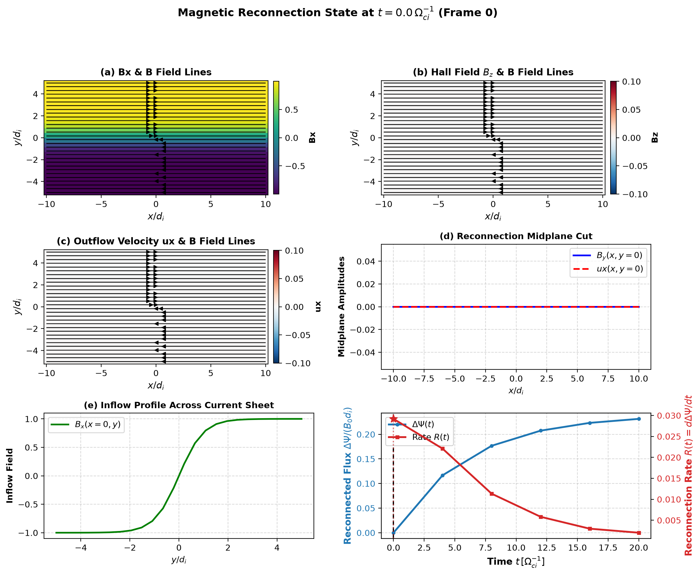
plot_peak_state automatically identifies the time of maximum reconnection rate and generates a 6-panel overview layout:

• (a) Outflow velocity or density with continuous streamlines + arrows

• (b) Hall magnetic field \(B_z\) with continuous streamlines + arrows

• © Reconnection outflow jets

• (d) 1D midplane cut \(B_y(x, y=0)\)

• (e) 1D inflow profile \(B_x(x=0, y)\) across the current sheet

• (f) Reconnection rate curve with a vertical indicator line for the current frame

fig, axes = reconn.plot_peak_state(series)
plt.show()

7. 2D Time Evolution

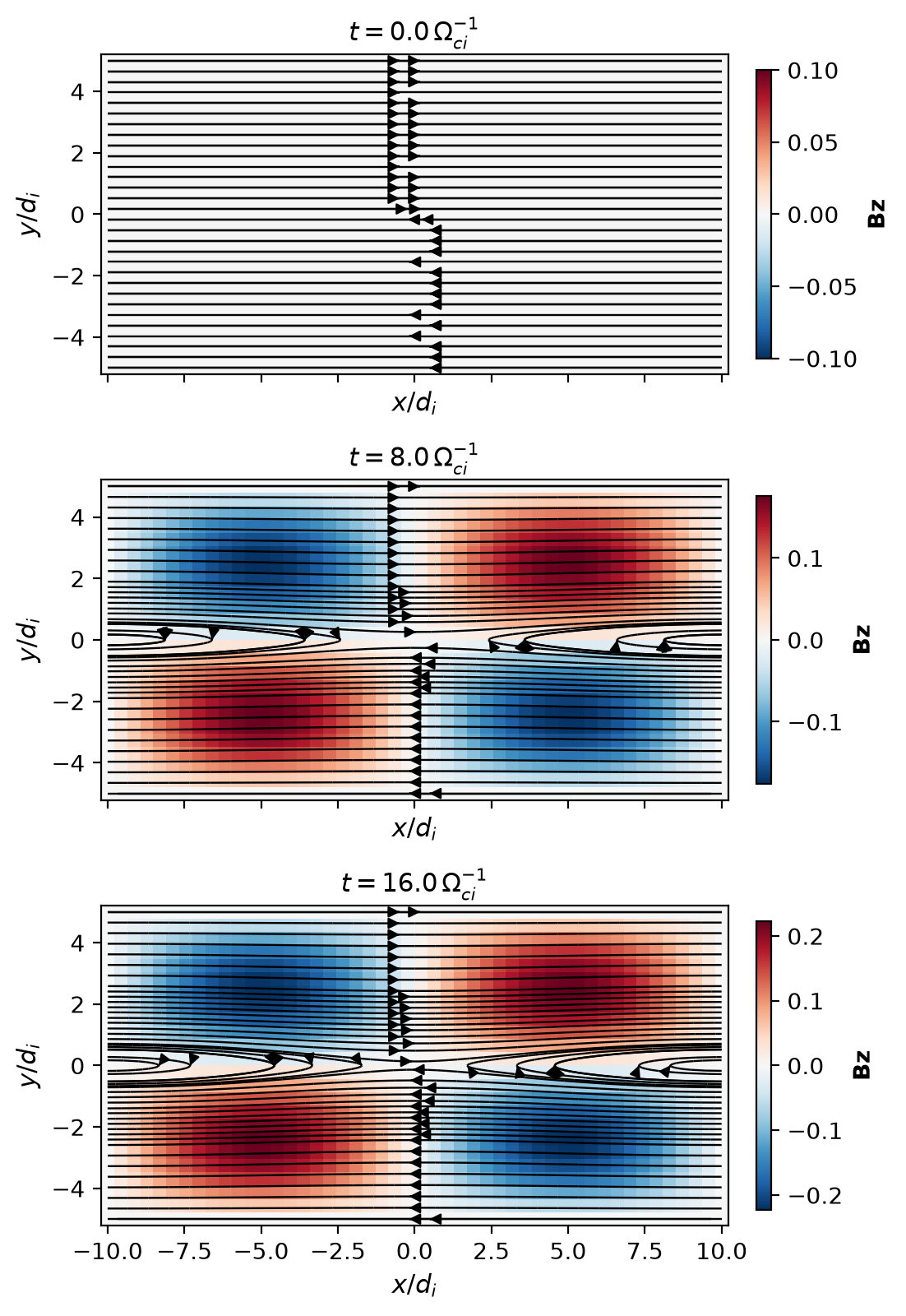
plot_2d_evolution visualizes the spatial evolution across key simulation times, illustrating current sheet thinning, island expansion, and magnetic topology changes:

fig, axes = reconn.plot_2d_evolution(
    series,
    var="Bz",
    times=[0.0, 8.0, 16.0],
    stream_field="B",
)
plt.show()

8. Cleanup

temp_dir.cleanup()
print("Cleaned up temporary synthetic data files.")

Cleaned up temporary synthetic data files.