ULF Waves

Ultra-low frequency (ULF) waves refer to waves within frequency range [0.001, 10] Hz. The name does not tell us anything about their physical origin, but simply observational fact. At Earth's magnetosphere, this frequency range overlaps largely with the MHD waves. This is the reason why early pioneers in space physics relied on MHD theory for large spatial and temporal scales to explain the physics behind these waves, albeit some deviations and deficiencies which require more refined models such as the Vlasov description.

Observation

ULF waves were originally called micropulsations or magnetic pulsations since they were first observed by ground magnetometers. ULF pulsations are classified into two types: pulsations continuous (Pc) and pulsations irregular (Pi) with several subclasses (Pc1–5 and Pi1–2) according to their frequencies and durations.^[1]

Notation	Period Range [s]
Pc1	0.2 - 5
Pc2	5 - 10
Pc3	10 - 45
Pc4	45 - 150
Pc5	150 - 600
Pi1	1 - 40
Pi2	40 - 150

[1]	The micropulsation division is based on their physical and morphological properties. The boundaries are not strict!

With respect to polarization, field line resonant ULF waves can be categorized into three modes: compressional ($\Delta B_\parallel,\, \Delta E_\phi$), poloidal ($\Delta B_r,\, \Delta E_\phi$), and toroidal ($\Delta B_\phi,\, \Delta E_r$). Here, $B_r$ ($E_r$), $B_\parallel$, and $B_\phi$ ($E_\phi$) are the radial, parallel (or compressional), and azimuthal components in the local magnetic field system, respectively. Referring to the basic MHD theory, the compressional modes are fast modes, whereas the poloidal and toriodal modes are Alfvén modes. The perturbed EM fields are related by $\mathbf{B}_1 = \frac{\mathbf{k}}{\omega} \times \mathbf{E}_1$. Think of a closed field line near the equatorial plane inside the magnetosphere: if the wave vector $\mathbf{k}$ is along the field line, i.e. $\mathbf{k} = (0,0,k_z)$, then there will be two cases for the EM field: poloidal where $\mathbf{E}_1$ in $\hat{\phi}$, $\mathbf{B}_1$ in $\hat{r}$ and toroidal where $\mathbf{E}_1$ in $\hat{r}$, $\mathbf{B}_1$ in $\hat{\phi}$. If the wave vector $\mathbf{k}$ is perpendicular to the field line, i.e. $\mathbf{k} = (k_x, 0, 0)$, since there is no $E_\parallel$ in MHD, we only have one option $\mathbf{E}_1$ in $\hat{\phi}$ and $\mathbf{B}_1$ in $\hat{z}$. A phase shift is allowed, and actually in real observations (e.g. THEMIS) it is rare that you can find B and E changing in-phase.

1. discrete magic frequencies

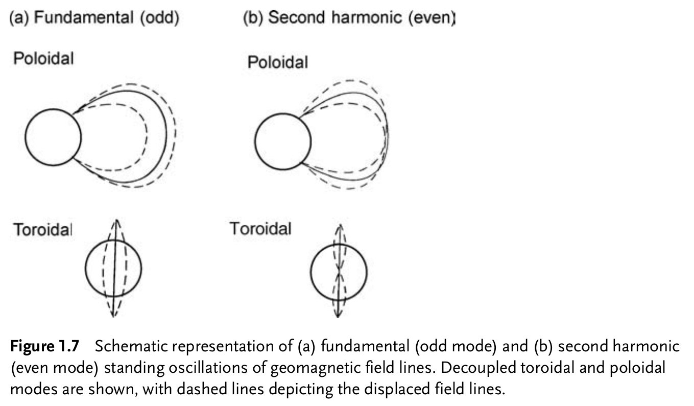
Field line resonance (FLR), which is phenonmenon about standing Alfvén waves excited on geomagnetic field lines (i.e closed field lines whose foot points lie in the ionosphere), are observed in the Pc5 range, with discrete frequencies at approximately 1.3, 1.9, 2.6, and 3.4 mHz.

2. Pc1 sudden impulses

• local noon-afternoon, easily detectable when following sudden impulses (SI) produced by sudden changes in the pressure of the solar wind plasma.

• A sudden compression of the magnetosphere by increased solar wind pressure causes maximum distortion of the quiet magnetospheric plasma near noon at high latitudes. It is on the fieldlines which thread this disturbed plasma that one is most likely to witness ULF emissions.

• Conversely, as suggested by Hirasawa (1981) sudden rarefactions of the magnetosphere would be expected to quench ULF wave growth by reducing the anisotropy and $\beta$ of the plasma.[rarefaction_ULF]

• delay of 1-3 mins between the occurance of SI and the onset of the ULF emission (ground-based magnetometers)[growth_rate]

• drive the trapped proton radiation, greatly enhanced eV energy range protons along the B field, and energization of keV range protons caused by betatron. (?) See Arnoldy+, 2005

Mode Identification

Given a background plasma state, a wave mode is a normal mode or eigenstate of the system. The eigen-value is usually taken to be the (complex) wave frequency $\omega$, with the real wave-vector $\mathbf{k}$ prescribed. The associated eigenvector is the set of fluctuating fields ($\delta\mathbf{E},\delta\mathbf{B}$) and plasma parameters ($\delta \rho, \delta\mathbf{u}, \delta P$ in the case of MHD or $\delta f_j(\mathbf{v})$ for kinetic waves where j stands for each species). Mode identification is the process of comparing the observed eigenvalue/eigenvector with the possible theoretical ones and finding the one which matches.

The practical implementation of mode identification is strewn with pitfalls and complications, including:

• There is usually a mixture, possibly phase-coherent, of modes and/or frequencies, rather than an isolated mode.

• Frequencies are often Doppler shifted by an unknown, or poorly known, amount.

• Wave vectors are difficult to determine from the one-(or few-) point measurements available from spacecraft.

• The mode eigenstate can depend sensitively on the wave vector, plasma $\beta$, and temperature anisotropy, as well as on the contributions of multi-species or non-Maxwellian kinetic features.

• The temporal resolution and accuracy of some measurements, notably those related to particle populations and plasma moments, are often insufficient or marginal. Some important species or sub-population may not be measured at all. The result is that either or both the background state or fluctuations are not accurately known.

• Wave amplitudes are often large (of order unity), implying nonlinear processes may be present and distort the eigenstate from its linear form, or give rise to intrinsically nonlinear eigenstates.

• Similarly, inhomogeneities can distort the wave propagation or eigenstate in ways which have largely been unexplored.

• As we have seen, the theoretical wave properties depend on the framework in which the theory is performed. There is a trade-off between the simplicity/dubious applicability of MHD or fluid treatments and the complexity associated with the infinite degrees of freedom of kinetic theory.

Our ultimate goal, is to build a tool for identifying wave modes automatically. Steven has already envisioned two types of models (decision tree, N-dimensional distance sampling) in 1996. 20 years later, people would find it more appealing to use machine learning.

Medeiros+ 2020 introduces a machine learning model for recognizing EMICWs from spectrograms. First she introduces the traditional approach of EMICW identification in near-Earth space via Fourier analyses of locally measured magnetic field data:

1. The Fourier power spectral density (PSD) in units of ${nT}^2 Hz^{−1}$ (B field) is plotted in a frequency-versus-time graph, yielding the so-called spectrogram.[field_comp]

2. Eye inspection of the wave packets' magnetic field amplitude, which in turn translates to (usually) localized, in both time and frequency, enhancements of PSDs relative to background values.

3. Computational techniques that interactively analyze the pixel intensities of the spectrogram's images against the background.

When wave packets are clearly distinct from the background, the interval can be considered as having a candidate EMIC wave event. Since the waves are in the 0.1–5 Hz frequency range, the data acquisition rate must be at least twice as high to resolve the wave packets.

Drivers

External Drivers

• periodic compressional fluctuations –> magnetopause surface waves

• Alfvénic fluctuations $\delta \mathbf{V}/ \mathbf{V}_A = \pm \delta \mathbf{B}/ \mathbf{B}_0$ direct excitation

• fast stream –> KHI on the magnetopause –> surface mode/waveguide^[2]

[2]	"guide" here refers to the fact that these modes are field-aligned, i.e. guided by the magnetic field. These are MHD Alfvén waves.

Electron and ion foreshocks are one typical ULF wave generation mechanism.

When the magnetopause can be described as a tangential discontinuity ($B_n = 0$), the MHD wave transmission is not efficient; when the magnetopause is a rotational discontinuity ($B_n\neq 0$), MHD wave transmission can occur over a wide range of incident angle and that the transmitted waves are usually amplified. The favored ULF wave range may lie within Pc5.

The correlation between solar wind speed and ULF power in the magnetosphere suggests that the Kelvin-Helmholtz instability (KHI) resulting from the velocity shear at the magnetopause may be a significant source of ULF wave energy. KHI studies were very active in the 1980s, but since then nothing really significant has been reached.

Boundary layer thickness –> over-reflection modes at the magnetopause Over-reflection occurs when the characteristic scales of the wave and the inhomogeneity are comparable, and may provide an efficient process for the extraction of energy from the magnetosheath to magnetospheric waveguide modes on the flanks during fast solar wind speed intervals. This may explain the production of discrete frequency ULF waves in the magnetosphere and statistical correlations between Pc5 power on the ground and solar wind velocity

Opinion: Alfvénic waves propagating along the magnetopause surface may develop into standing Alfvén waves on the boundary due to reflection from the conjugate ionospheres (i.e. Kruskal-Schwarzschild modes). The surface waves are likely due to magnetopause displacements as a result of local pressure perturbations in the magnetosheath, while the eigenfrequencies of the standing modes are determined by the magnetopause geometry and are strikingly similar to the Samson "magic" frequencies. This combination of conditions suggests that the oscillations are more likely due to Kruskal-Schwarzshild modes than solar wind pressure perturbations or the KHI at the flanks.

Pressure Variation

1. Solar wind dynamic pressure pulses identified by

• depressed magnetic field strength

• enhanced plasma density

• compressed magnetosphere

• enhanced magnetic field strength observed by "static" satellites

Southwood and Kivelson has described the basic picture of pressure viriations pretty well: < The magnetosphere is not rigid; the plasma motions due to compression are not necessarily in phase. If a change in external pressure takes place on a time scale shorter than the time taken by a MHD wave to travel through the magnetospheric cavity (~ 10 min), the magnetopause acts as a source of a compressional MHD signal that propagates through the system. As well as communicating the new equilibrium conditions, the signal can excite transient responses, for example normal modes. The magnetosphere as a whole can ring (a global compressional mode response) or ringing may be confined to certain selected shells (field resonance). Even where the global mode is not excited there is still a response away from the resonant shell. In this case the response will more directly reflect the form of the applied pressure changes as the signal will not be contaminated by the presence of an oscillatory transient associated with a normal mode response.

There is also an ionospheric response, but I don't know the details.

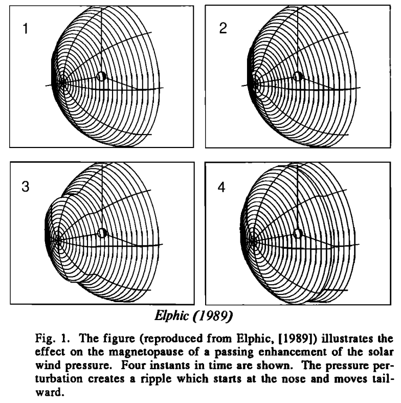
The typical pressure perturbation, be it periodic or an impulsive or stepwise change, will exhibit some structure, e.g., a front or a series of phase fronts that moves systematically away from the Sun. The schematic figure shows a series of pictures illustrating the motion of an isolated pressure pulse over the magnetopause. A ridge moves over the magnetopause away from the subsolar point. In the sketch there is a single front within which the magnetopause moves in and out producing a compressional change of limited extent. As the compression sweeps around the magnetopause the pressure perturbation imposed on the magnetosphere has both a characteristic spatial scale size, L, and time, T, linked by the relation

$T \approx L / U$

where U is the speed along the boundary. We must allow for a spatial structure that is imposed by the perturbation and it is also clear that the motion of the perturbation is both along and across the magnetic field. As mentioned later in the paper, the scale length perpendicular to the field is of some significance in determining the type of magnetospheric response. We shall parametrize the variation imposed at the boundary by assuming that a given perturbation may be made up of a collection (potentially infinite) of spatial Fourier components and we shall describe the response to a specific Fourier component. In a similar spirit we shall use Laplace transforms to describe the temporal structure of the perturbation. However, we shall need to switch from frequency domain to time domain as we outline the types of system response and so we shall have to treat the variation more rigorously in time than in space.

One possible physical process is that the pressure pulses first strike the magnetopause and then launched sunward moving boundary waves on the magnetopause.

2. Pressure pulses can also be generated in the foreshock region as a result of the instability due to ions backstreaming from the shock.

• The density perturbations in this case often have a positive correlation with magnetic fields.

The impact of pressure pulses on the magnetopause is known to be related to traveling convection vortices, flux transfer events,and auroral activities.

Internal Drivers

Within the magnetosphere, there are two possible mechanics:

• drift-mirror instabilities (?) due to high $\beta$ pressure anisotropies

• drift-bounce resonance (?) with trapped energetic ions

From observation, $T_\perp / T_\parallel > 5$ is practically treated as high anisotropies.

strongly compressional, high azimuthal wave number m, attenuated on the ground.

From the energy perspective, it is important to estimate how much energy FLRs deposit into the ionosphere, the energy dissipated into the ionosphere via Joule heating.

Wave Generation and Propagation Mechanisms

Menk, 2011的综述文章只能硬着头皮看。太多从文章中抄出来的经验性总结了,对于入门新手极不友好。

David Southwood, Margy Kivelson, and Steven Schwartz have done a lot in this field.

Quote from Steven Schwartz's paper:

For most aspects of space plasmas, and certainly for the waves observed in the magnetosheath, fluid-based descriptions of any kind are inadequate, particularly under the $\beta > 1$ conditions found there. And we have not yet considered complications due to inhomogeneity and nonlinearity!

The propagation of magnetospheric ULF plasma waves has been described usually usually in the context of standing shear Alfvén mode field line oscillations with low azimuthal wavenumber that are driven by energy coupling from incoming compressional fast mode waves.

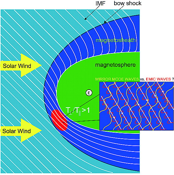
Downstream of the quasi-perpendicular portion of the bow shock, solar wind protons and heavier ions (helium ions) are preferentially heated in the perpendicular direction to the magnetic field.^[3] This heating creates strong temperature anisotropies which lead to intense wave growth. Several kinds of instabilities can be triggered: mirror mode instability and L-mode electromagnetic ion-cyclotron instability (EMIC). The development of pressure anisotropy can have a significant stabilizing effect on the dynamic evolution, while a reduction of the anisotropy as expected from microscopic, anisotropy driven instability reduces this stabilization and brings the evolution closer to the isotropic case Birn+1995. EMIC mode dominates when the plasma β is low while mirror mode dominates when the plasma β is high. Slow modes may also be present within the plasma depletion layer^[4], although they are expected to suffer strong damping. These instabilities, if exist, allow energy transfer from the plasma to the electromagnetic field and creates the waves via reducing the temperature anisotropy and creating magnetic field oscillations for the mirror instability. So in a sense the instability initiates the waves, and the waves are these oscillations once they are "established" in the plasma.

[3]

Yuxi provides me with a nice starting point to think about this. The 1st adiabatic invariant, i.e. magnetic moment $\mu_m = \frac{1}{2}m v_\perp^2 / B$ is almost conserved if the gyromotion is not violated. Across the quasi-perpendicular shock, the strength of the magnetic field increases, so the perpendicular thermal velocities must increase to maintain the magnetic moment. Therefore the perpendicular direction is preferentially heated downstream of the shock. For example, if the B field is increased by a factor of 2, then the ion perpendicular thermal velocity should increase by a factor of $\sqrt{2}$, and the ion perpendicular pressure should also increase by a factor of 2? Never or less, keep in mind that in CGL theory we need at least 1 quantity from downstream besides the full upstream information to determine the downstream anisotropy (see more in the shock note).

[4]	The plasma depletion layer (PDL) is a layer on the sunward side of the magnetopause with lower plasma density

and higher magnetic field compared to the corresponding upstream magnetosheath value.

Isotropic MHD waves

Fast/Slow wave

In linearized ideal isotropic MHD, fast, slow, and Alfvén mode are all linearly dispersive, i.e. phase velocity independent of the wavelength.

compressive, $P_B$ and $P_t$ in phase for fast mode and in anti-phase for slow mode

fast mode nearly isotropic for phase speed, while the slow mode is strongly guided by magnetic field direction

Theoretically, slow and fast MHD waves usually are quickly damped in collisionless plasmas with moderate to high plasma β (Barnes, 1966), leaving only outward propagating Alfvén waves.

Fast mode: ion/ion right-hand resonant

Alfvén wave

non-compressive, travels along the magnetic field, i.e. group velocity is field-aligned, $\delta{u} \parallel \delta{\mathbf{B}}$

ion/ion left-hand resonant

Entropy wave

There is a 4th zero-frequency mode from HD/MHD theory, referred to as entropy mode, which is often ignored. It is a compressional wave (i.e. fluctuations in density) traveling at bulk velocity in which the internal energy and velocity remains constant. It represents a spatially structured medium in static equilibrium, being characterized by the sole density variation with the other variables being kept constant.

$\frac{Ds}{Dt} = \frac{\partial s}{\partial t} + \mathbf{u}\cdot\nabla{s} = 0$

where entropy density $s$ is defined as

$s = n \log\Big( \frac{T^{3/2}}{n} \Big)$

Anisotropic MHD waves

Chew, Goldberger, and Low (CGL) theory

In CGL theory, we obtain the relationship between density and magnetic field fluctuations

$\frac{\delta n}{n} = \Big( \frac{P_\perp \sin^2\theta}{n m_p} \Big)^{-1}\Big[ \frac{\omega^2}{k^2} - \frac{B^2}{\mu_0 n m_p} - \frac{P_\perp}{n m_p} + \frac{P_\parallel \cos^2\theta}{n m_p} \Big] \frac{\delta B}{B},$

where $m_p$ is the proton mass, $\theta$ is the angle between the wave vector $\mathbf{k}$ and the magnetic field, and $P_\perp$, $P_\parallel$ are the perpendicular and parallel thermal pressures.

This a general relationship between the density and magnetic fluctuations for the slow and fast modes. It can be shown that the fast mode always gives positively correlated δn and δB. The firehose instability arising from this mode will also induce in-phase density and magnetic field fluctuations, at least in its linear stage. The intermediate mode with a dispersion relation

$\frac{\omega^2}{k^2} = v_A^2 \Big( \frac{P_\perp - P_\parallel}{B^2/\mu_0} + 1 \Big) \cos^2\theta$

is not involved with the perturbations so that δn = δB = 0 across this mode as in the ordinary MHD theory. Here $v_A$ denotes the Alfvén speed.

If we take $\theta \sim 90^o$, the general relation can be simplified to

$\frac{\delta n}{n} = -\Big( 1 + \frac{2}{\beta_\perp} \Big) \frac{\delta B}{B}$

for the slow mode. Don't mess this up with the slow wave in isotropic MHD, where it cannot propagate in the perpendicular direction!

Firehose instability

The Alfvén wave remains transverse but becomes the firehose instability for $P_{0\parallel} > P_{0\perp} + B_O^2/\mu_0$.

ion/ion nonresonant

Fast mode

very similar to the isotropic case

Mirror instability

The slow magnetosonic mode "becomes" the mirror instability for anisotropies satisfying

$\frac{P_{0\perp}}{P_{0\parallel}} > 6 \Big( 1 + \frac{B_0^2}{2\mu_0 P_{0\perp}} \Big) = 6 \Big( 1 + \frac{P_B}{P_{0\perp}} \Big).$

The lowest threshold corresponds to wave-vectors perpendicular to the background magnetic field.

There is an important difference between slow mode and mirror mode. Southwood & Kivelson, 1993 and Hasegawa 1969 derived under the CGL framework that even though the slow mode and mirror mode shares the antiphase relation between thermal pressure (or more exactly, perpendicular thermal pressure) and magnetic pressure, they are not the same: the CGL fluid theory predicts oscillations in the perpendicular direction for mirror mode when the fluid instability conditions is not met, while the slow mode cannot propagate in the perpendiclar direction at all! Schwartz's 1997 review paper did not make this point clear. And again keep in mind that even setting $P_\perp = P_\parallel$ we cannot recover isotropic MHD equations from CGL equations (See Hunana+, 2019)!

Mirror Mode

History

Back to the 1960s, people found a new type of instability when conducting experiments on ohmic heating of a plasma by means of a current directed along an intense magnetic field. It was early recognized that this mode for being excited require a transverse pressure (or temperature) anisotropy.[anisotropy_source] Rudakov & Sagdeyev explained its physics using fluid approach in a paper written in Russian.

This instability has generally been called mirror instability because a loss cone distribution inherently creates such an anisotropic pressure. It is actually not quite relevant in the mirror fusion machine because it has never become a high-β machine. For a complete theoretical derivation, I must read the classical Hasegawa paper.

In 1967, Masayoshi Tajiri derived a kinetic description of the mirror mode when considering the propagation of linear (i.e. small amplitude) MHD waves in a collisionless plasma under homogeneous background. The key difference when compared against the CGL fluid approach is that is mirror mode is shown to be an non-oscillating mode with vanishing real part of the frequency, which means that it has zero frequency in the plasma rest frame. Under proper conditions, the non-oscillating wave causes the mirror instability in the direction nearly perpendicular to a magnetic field.

In 1969, Akira Hasegawa extend the kinetic theory to a nonuniform medium which takes magnetic field gradient and finite-Larmor-radius effect into account. If we consider finite Larmor radius (FLR) effect, then the mirror mode becomes a drift mirror instability, which leads to the $r^2_L \nabla^2$ term in the drift velocity. The Larmor radius is much larger for ions than for electrons, so the drift will create charge separation and electric fields. If we consider inhomogeneity, the non-propagation is also no longer true.

Since the magnetic field in mirror modes forms extended though slightly oblique magnetic bottles, low parallel energy particles can be trapped in mirror modes and redistribute energy. Such trapped electrons excite banded whistler wave emission known under the name of lion roars and indicating that the mirror modes contain a trapped particle component while leading to the splitting of particle distributions into trapped and passing particles. The most amazing fact about mirror modes is, however, that they evolve in the practically fully collisionless regime of high temperature plasma where it is on thermodynamic reasons entirely impossible to expel any magnetic field from the plasma.^[5] The fact that magnetic fields are indeed locally extracted makes mirror modes similar to “superconducting” structures in matter as known only at extremely low temperatures. Of course, microscopic quantum effects do not play a role in mirror modes. However, it seems that all mirror structures have typical scales of the order of the ion inertial length which implies that mirrors evolve in a regime where the transverse ion and electron motions decouple. In this case the Hall kinetics comes into play.

[5]

how should I interpret this sentence? Mirror modes cause some structuring of the plasma thus generating a state of lower entropy than the initial state. Moreover, the plasma is ideally conducting which implies that plasma and magnetic field are frozen and cannot be separated from each other. One therefore has to find a mechanism which distorts both the frozen-in state and leads to lower entropy without violating the second theromodynamics law, in other words, the lower entropy state has to be a state of reduced free energy.

Ambiguity about mirror modes

Mirror mode oscillation is the lowest frequency perpendicular magnetic excitation in magnetized plasma. In principle mirror modes are some version of slow mode waves, i.e. the density and magnetic field fluctuations are in strict anti-phase. Fluid theory, however, does not give a correct physical picture of the mirror mode. As the lowest frequency mode it can be expected that mirror modes serve as one of the dominant energy inputs into plasma. This is however true only when the mode grows to large amplitude leaving the linear stage.Treumann+, 2004

At such low frequencies, on the other hand, quasilinear theory does not apply as a valid saturation mechanism. Probably the dominant processes are related to the generation of gradients in the plasma which serve as the cause of drift modes thus transferring energy to shorter wavelength propagating waves of higher nonzero frequency. This kind of theory has not yet been developed as it has not yet been understood why mirror modes in spite of their slow growth rate usually are of very large amplitudes indeed of the order of $|B/B_0|^2\sim O(1)$.

Quasilinear theory predicts the reduction of the initial ion pressure anisotropy towards stabilization up to a minimum required for keeping the final state. Though this seems to be quite reasonable, the validity of the theory is strongly questionable because the mirror mode is a non-oscillatory wave mode of small growth rate such that averaging over the period of the wave oscillation becomes spurious. There is plenty of time for other higher frequency instabilities to develop feeded by either the plasma anisotropy or by the plasma gradients self-consistently generated by the linear mirror mode itself in the plasma. In the first case one expects ion cyclotron instabilities to arise, in the second case short-wavelength high-frequency drift instabilities should evolve rapidly destroying the mirror mode.

More questions arise when thinking about mirror modes.

1. In plasma with temperature (pressure) anisotropy $A = T_\perp/T_\parallel > 1$ required for mirror modes to exist, Alfvén waves remain stable and cannot be excited unless some peculiar mechanism (like fast field aligned ion beams propagating across the plasma or local field-aligned electric potential drops serving as sources of Alfvén waves) is at work. Neither of such mechanisms exists in the magnetosheath.

2. Observations show that the structures do not appear isolated but in chains of many closely located magnetic depressions separated by intense magnetic walls.

3. Their magnetic field polarization is entirely parallel with negligible transverse magnetic components, indicating that

their phase velocities are very close to being perpendicular which is in striking contrast to Alfvénic structures where the compressional component can be neglected.^[6]

4. Investigation of the particle components inside the mirror structures suggests that they contain trapped particle components which are the signature of a mirror configuration which confines the low energy component to the region of magnetic field depression. This low energy zero parallel velocity component is crucial in formation of mirror modes (as has been realized first by Southwood and Kivelson, 1993) since it is the one which is in resonance.

[6]

This is one of the most confusing point when I thought that mirror mode was just one kind of slow mode. Slow mode in MHD propagate preferably in the parallel direction, which is the opposite of mirror mode. This strange property also indicates that in GSM coordinates of the magnetosheath, we shall look at Bz perturbation for mirror mode, especially in low latitude regions.

From this discussion it follows that the mere existence of mirror mode structures is a somewhat strange fact, in particular because in high temperature plasma a large number of oscillation modes like drift waves may arise which will fatally affect the evolution of mirror modes. However the existence of mirror bubbles suggests that they themselves represent a lowest frequency quasi-stationary mode that may evolve in a high temperature plasma leading to a distinct spatial structuring of the plasma both in the magnetic field as in the plasma pressure and densities. Mirror modes in their nonlinear state thus represent a state of minimum free energy in an anisotropic high temperature plasma with excess transverse temperature. Since structures of this kind have very low phase velocity $\omega/k \approx 0$ in the plasma frame they are subject to convection along with the plasma itself. Their frequency in the spacecraft frame is given by $\omega_{sc}\approx \mathbf{k}\cdot\mathbf{v}$ causing distinct frequency power spectra $P(\omega_{sc})$ which map the wavelength spectrum $P(\mathbf{k})$ of the mirror modes into the frequency domain.

Properties

See a nice review in the section "Summary of linear theory" in Treumann+, 2004.

The energy source of the mirror mode is the pressure (or temperature) anisotropy of the ions. Mirror mode instabilities described by the kinetic theory produce anticorrelated density and magnetic field fluctuations following

$\frac{\delta n}{n} = -\big( \frac{T_\perp}{T_\parallel} - 1 \big)\frac{\delta B}{B}$

for a bi-Maxwellian plasma, where δn and δB are perturbations in the background plasma density n and magnetic field strength B.

Interestingly, the mirror mode is unstable in kinetic theory for temperature anisotropies satisfying

$\frac{T_\perp}{T_\parallel} > 1 + \frac{1}{\beta_\perp},$

which is similar to that found in mixed kinetic-fluid treatments, and disagrees by a factor of 6 with the result in CGS approximations given above. This relation confirms that the mirror mode is favored by large $\beta$. There is another commonly used form

$\beta_\perp \Big(\frac{T_\perp}{T_\parallel} - 1 \Big) > 1.$

As this threshold is reached, the first unstable mode has a wave vector $\mathbf{k}$ which is nearly perpendicular to $\mathbf{B}_0$. As the anisotropy is increased, however, the most unstable mode shifts to more oblique $\mathbf{k}$'s, reaching $\theta_{kB_0} \simeq 60^o$ for $T_\perp / T_\parallel \ge 2$. Warm/hot electrons modify the instability threshold to some extent, and decrease the growth rate.

From one AMPTE IRM observation in the magnetosheath (Treumann+, 2004) , I see a periodic oscillation of ~20 s in the magnetic field. The spatial scale of mirror modes is the order of $\lambda_\perp \sim \lambda_i$ ($\sim 10^2$ km), which is also comparable with the gyroradius $r_{ci} = v_{i\perp}/\omega_{ci}$.[mirror_scale]

Song+, 1994 proposed a quantity called Doppler ratio for distinguishing the mirror and slow modes:

$D = \frac{|\delta \mathbf{v}|^2/v_0^2}{|\delta \mathbf{B}|^2/B_0^2}$

where $\delta\mathbf{v}$ and $v_0$ are the perturbed velocity and magnetitude of the background flow velocity. This represents the perturbation power in the velocity versus that in the magnetic field. In general, slow waves have perturbations in both the velocity and magnetic field, but mirror mode fluctuations do not produce significant velocity perturbations. Therefore if the flow is sub-Alfvénic, the Doppler ratio is greater than 1 for quasi-perpendicular slow modes and should be much smaller than 1 for mirror modes. See Appendix A in that paper for some more derivations.

$\delta\mathbf{B} / \bar\mathbf{B} \sim 0.1$ or more, and is almost linearly polarized along the ambient field.

Electromagnetic Ion-Cyclotron Waves (EMICWs)

Ion-cyclotron waves are driven by an ion temperature anisotropy $T_\perp / T_\parallel > 1$, as is commonly found in the magnetosheath. The instability is strongest for parallely propagating modes ($\theta_{kB_0} \sim 0^o$) and is weakly dependent on the ion $\beta$. If being called as Alfvén ion-cyclotron mode, as in Schwartz's 1997 review paper, then is left-hand polarized at parallel propagation in the plasma rest frame, being cyclotron resonant with the ions. Maximum growth corresponds to wave numbers $k \simeq 0.5 - \omega_{pp}/c$, where $\omega_{pp}$ is the proton plasma frequency. However, ion-cyclotron waves may have different polarizations! There have been observations about left-hand polarized, right-hand polarized, and linear polarized EMIC waves, probably distributed among different MLT regions as well as latitudes.

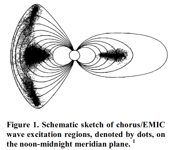
Zhang+ 2017 provides a nice overview of EMICW, even though the paper itself is about MMS observation. Under a dipole-like magnetic field configuration in the Earth’s inner magnetosphere, the excitation region of EMIC waves is usually on or near the magnetic equatorial plane, where

• the magnetic energy per particle is lower and thus

• the growth rate of waves is larger due to the greater plasma density and weaker magnetic field strength (minimum B regions).[EMIC_region]

EMIC waves are preferentially generated in regions where hot anisotropic ions and cold dense plasma populations spatially overlap, e.g.

• where the ring current overlaps the outer plasmasphere and plasmapause

• the "edges" of plasmaspheric drainage plumes.

Physical processes that can lead to warm plasma temperature anisotropies can be broadly categorized as two types: those that change the overall temperature (energizing processes) preferentially in the perpendicular direction, and those that keep the overall temperature constant (nonenergizing processes) while redistributing particle energies between the perpendicular and parallel directions.McCollough+, 2010

1. Drift-shell splitting. In any dipole-like field that has been distorted by the solar wind, conservation of the first and second adiabatic invariants as particles drift from the nightside to the dayside leads to drift shell splitting: the particle population spreads in L shell as a function equatorial pitch angle $\alpha_{eq}$, with higher $\alpha_{eq}$ particles found at higher L shells on the dayside. If the particle flux is decreasing as a function of L, temperature anisotropies emerge with no energy input into the system.

2. Shabansky orbits (a non-energization mechanism). If the dipole-like field is significantly distorted, near-equatorial particles at higher L shells will execute their bounce motion entirely in one hemisphere.

3. Compression, which is often driven by a sudden, large increase in the solar wind dynamic pressure. When the magnetosphere compresses at a slow enough rate to keep all adiabatic invariants conserved, adiabatic energization Olson & Lee, 1983 occurs. This is an energizing process, since the locally increasing field increases both the perpendicular and parallel energy of the particles. However, the perpendicular energy increases to a greater degree than the parallel energy, which makes the resulting distribution anisotropic. Similarly, by preserving the first adiabatic invariant, convection electric fields provide perpendicular energy as warm ions are transported radially inward Summers+, 1998. Other processes can lead to radial transport as well, including coherent response to shocks in the solar wind, interactions with solar wind–driven ULF waves, and drift scattering by storm time Pc5 waves.

Newly excited EMIC waves are often transverse and left-hand polarized, consistent with the direction of ion gyration in the magnetic field. After being generated, EMIC waves can be guided along the magnetic field lines and propagate from the source region to other magnetic latitudes. In the case of the equatorial source region, they propagate from the equatorial plane to higher latitudes. Combined Release and Radiation Effects Satellite (CRRES) EM field data (covering only MLT = 14:00 – 18:00) shows that the directions of the energy propagation (i.e., Poynting vector) of EMIC waves are unidirectional when |MLAT| > 11° but they are bidirectional in the MLAT range of [-11°, 11°] in the inner magnetosphere. Depending on their frequency w.r.t. the local ion gyrofrequencies such as $f_{He^+}$, some waves are well guided along the field lines and can generally propagate to the ground. Some waves may even experience a polarization reversal where the wave frequency f is equal to the crossover frequency $f_{co}$ (???) during their higher-latitude propagation and then be reflected where f equals the bi-ion hybrid frequency $f_{bi}$ (???) at an even higher latitude. As a result, their polarization is crossed over from a left-hand to a right-hand or linear mode. These waves could undergo multiple equatorial crossings along magnetic flux tubes without a large radial or azimuthal drift. Because of their successive passes through the equatorial wave growth region, the waves are expected to be drastically amplified by continuing to obtain energy from the energetic protons. Nevertheless, Horne and Thorne found that, in the absence of density gradients, significant wave amplifications can only occur on the first equatorial pass because wave normal angles become large after the initial pass. Horne and Thorne concluded that wave damping by thermal heavy ions also makes it impossible for the same EMIC wave packet to bounce through its source region multiple times. But, a consensus about the wave propagation and reflection has not been reached.

A dissertation on the THEMIS observation of EMIC waves in the Earth’s Magnetosphere

Ion-cyclotron wave can be derived in a Hall MHD framework: it comes as one of the two solutions from the dispersion relation, the other being electron-cyclotron wave, more commonly known as whistler wave. The development of the ion cyclotron wave is usually described by the standard quasi-linear theory in which the unstable distribution equilibrates through a spatially smooth process of velocity space diffusion.

The waves are generally believed to be generated in the equatorial magnetosphere by

• ion-cyclotron resonance with unstable distributions of energetic ring current ions during the recovery phase of magnetic storms

• during compressions of the day-side magnetopause (??? Thorne 2013)

At Earth, EMICWs are typically observed in Pc1 and Pc2 range. In the outer radiation belt, the frequency typically ranges between 0.1 to 5 Hz. The characteristic fine structure appearance of ‘pearl’ Pc1 waves was attributed to dispersive field-aligned wave packet propagation in the LH ion mode on successive bounces between hemispheres. However, this still lacks observation support. Spacecraft measurements have shown that EMICW propagation is almost exclusively away from the equator at latitudes greater than about 11◦, with minimal reflection at the ionosphere.

The preferential region of occurrence of EMIC waves is known to be the afternoon magnetic local time (MLT) sector from ∼12:00 to ∼18:00 MLT in the region near the plasmapause and the plasmaspheric plume.

Recent modeling efforts have focused on clarifying the locations and conditions for EMICW generation, including the effect of heavy ion populations, and explaining the modulated appearance of wave packets. However, there is no clear consensus on a dominant mechanism. These are important questions since EMIC waves may control the precipitation of energetic ions and relativistic electrons.

Plasma density is one of the most important parameters controlling EMIC wave generation. Complexity arises when we need to consider both thermal and cold plasma.

Gamayunov and Khazanov, 2008 using a global RCEMIC simulation model suggests that suprathermal plasma plays a role in destabilizing the more energetic ring current and/or plasma sheet distributions to a high energy anisotropy. It also suggests that for best data comparison the EMICW source is located at the equator and that waves reflect at off-equatorial latitudes at the bi-ion hybrid frequencies in conjugate hemispheres.

self-written model, no name, ray-tracing equations in plasma

particle scattering and trapping by waves. Hmm, I'm not familiar with these at all.

我看到几个2Dshock模拟，都是选一个平行磁场一个垂直磁场（即GSM中的XZ平面）做的。EMIC波主要平行于背景磁场方向传播，所以最常见的确认方法是看波的横截面中的磁场扰动周期。在老仪器中我猜测量磁场的磁强计比较靠谱，而测量电场的设备误差很大，所以以前的观测主要通过磁场扰动来确认。但像THEMIS以后电场的测量精度也上来了，所以也可以通过看电场扰动来确认。毕竟是电磁波，理论上无论是啥偏振，扰动的频谱都应该是一致的。

$\delta\mathbf{B} / \bar\mathbf{B} \sim 0.03$ from my 2D Vlasiator simulation. Waiting for Dr. Soucek's response for the threshold he used for Cluster data!

Mirror Instability & Ion Cyclotron Instability

Already, early observations in the 1970s have shown that the magnetosheath is populated by intense magnetic field fluctuations at time sclaes from 1 s to 10 s of seconds. Later research based primarily on data from ISEE and AMPTE satellites has shown that the mirror mode waves and kinetic Alfvén-ion cyclotron (AIC) waves, or EMIC waves constitute a large majority of magnetosheath ULF waves. The ion cyclotron instability responsible for the generation of AIC waves often grows under the same conditions as the mirror instability and in the linear approximation should dominate in lower β plasmas. The mirror instability, on the other hand, should dominate in high ion β plasmas (Lacombe & Belmont, 1995). Since the initial confirmation of the existence of mirror modes in the Earth's magnetosheath, they have been observed throughout the heliosphere. A long-standing puzzle in space plasmas is the fact that mirror modes are often the dominant coherent magnetic structures even for low β plasmas.

People tried to find an answer to this puzzle. A bunch of studies in late 1980s and early 1990s (e.g. [Gary+]) argued that the presence of $He^{++}$ tends to increase the EMIC threshold while the mirror mode growth is less affected by the presence of $He^{++}$ ions. Yoshiharu Omura's student Shoji+2009 presented another possibility with hybrid PIC simulations that even though EMIC modes have higher linear growth rate, they saturates an an earlier stage than the mirror modes, especially in higher dimensions (by comparing 2D and 3D results), so that mirror mode waves can gain more free energy from temperature anisotropy.

During the nonlinear stage:

In the 3D case mirror mode coalescence is much more rapid. Because of this rapid change, electric fields are induced, and the energy of the electromagnetic fields is converted to the thermal energy of particles. At the end of the nonlinear evolution, the structures in the 3D model collapse. On the other hand, in the 2D model, the large structure remains. Through the nonlinear evolution resulting plasma turbulence in the 3D model, the particles are heated by the induced electric field in the perpendicular direction. They are diffused in pitch angles to parallel direction and to make beta in the parallel direction larger.

简单点说就是：

1. 虽然离子回旋波在线性阶段长得快，但它很容易饱和并且空间自由度越高饱和得越快。在饱和以后就不增长了，进入非线性阶段。而磁镜波虽然增长率小，但是需要很长时间才能达到饱和。

2. 三维情况下模式合并的情况与二维情况下不同。

Spatial Distribution

1. AIC/EMIC are found predominantly near the bow shock and in the plasma depletion layer^[4] (Song+, 1994, Hubert+, 1998).

2. Mirror mode waves dominate in the central and downstream magnetosheath but can occur immediately downstream of quasi-perpendicular shocks too. Hubert+, 1989

3. ULF waves are generally stronger in the dayside magnetosheath.

4. More frequency EMIC wave occurrence during quasi-parallel shocks.

Field Line Resonance

The resonant mode coupling is one of major physical processes in the space plasmas including the magnetic reconnection and collisionless shock wave. The field-line resonance describes the resonant interaction between compressional fast waves and shear Alfvén waves in a non-uniform plasma such as the Earth magnetosphere. The concept of this resonant mode coupling was first outlined by Tsutomu Tamao in 1961 and later discussed in his seminal paper on hydromagnetic coupling resonances (Tamao, 1965). Experimental work by John Samson+ (1971) made resonant mode coupling the current paradigm of planetary magnetospheric ULF-wave research.

We learned from ground, ionospheric, and space observations about the existence of only one or at least a few resonant field line vibrations (i.e. eigenoscillations) in the Pc5 range in the magnetosphere. As the Alfvén velocity is varying in the radial direction and as most sources of magnetospheric hydromagnetic waves are broadband sources, the resonance condition can be matched at an infinite number of geomagnetic field lines. Thus, every field line should be in resonance for a broad enough energy source. Thus the observational fact of "magic" frequencies requires a magnetospheric frequency selection rule. [Kivelson and Southwood, 1985] suggested that perturbations due to a broadband source at, e.g., the magnetopause first couple to the discrete eigenoscillations of global compressional eigenmodes. These narrow band compressional modes then couple to Alfvénic perturbations due to the field line resonance mechanism. The global modes thus select the frequency components participating in the resonant coupling. An alternative way of selection has been proposed by [Fujita+, 1996], who demonstrated that the K–H instability at the surface of a non-uniform magnetospheric plasma introduces dispersive properties of the unstable waves, which then gives rise to a narrower source spectrum. Thus, the field line resonance concept as outlined above is able to explain the major features of observed resonant ULF pulsations in the terrestrial magnetosphere.

Possible mechanism

• MHD waveguide

• MHD cavity modes

In fact, the coupling of cavity or waveguide eigenmodes to FLRs may explain how discrete spectra are produced across a range of latitudes, including at the "magic" frequencies. The global cavity modes may be responsible for the appearance of ULF signals with multiple discrete spectral peaks at the "magic" frequencies and spanning a range of latitudes, but it is hard to detect with satellites. (This is interesting, the Archer+ 2019, 2022 papers handle this.)

Thinking about fast modes propagating in dayside magnetosphere trapped or guided by the field lines and boundaries within. Cavity modes assume that you have a closed system. It can produce discrete azimuthal wave numbers. Waveguide modes assumes open-ended boundary conditions. It allows continuous azimuthal wave number spectrum.

In the 1970s, KHI is cited as the source of compressional energy required for the excitation of FLRs. However, later people have found that the same can be triggered by solar wind dynamic pressure fluctuation. Simultaneous measurements are applied to show that periodic fluctuations in the solar wind dynamic pressure drives ULF pulsations in the magnetosphere. A one‐to‐one correspondence was observed between the solar wind number density oscillation frequencies and oscillation frequencies in dayside magnetic field measurements from the GOES satellite. Even magnetotail lobe oscillations have been associated with upstream dynamic pressure fluctuation. One statistical study in 2009 by Viall+ is trying to argue that 50% of the ULF waves in the magnetosphere is driven by upstream solar wind dynamic pressure fluctuations.

In SouthwoodKivelson1990, they provided a theoretical work on the FLRs and cavity mode as magnetospheric response to solar wind dynamic pressure changes.

Glassmeier+, 1999 presented a nice review on the FLR theory. To fully understand the basis of the theory, I also need to read Theory of Hydromagnetic Waves in the Magnetosphere.

Earliest Discovery

Tsutomu Tamao, a physicist at Tohoku university, published a canonical paper in a local journal. It does not matter where to publish your work; it matters if you really do your work.

In his seminal approach to the problem of the propagation and coupling of hydromagnetic waves in non-uniform media, Tamao 1965 discussed the time harmonic wave propagation in a dipole magnetosphere in a linear approximation. Dissipation due to collisions, that are Ohmic and viscous effects, is neglected as well as electron inertia. In the following we will outline Tamao’s treatment for historical reasons and to demonstrate how detailed his early study really was.

The equation for the velocity perturbation component transverse to the ambient dipole field is given by

$\nabla^2 \Big( \mathbf{C}\times\hat{\eta} - i\frac{\omega}{\Omega_i} \Big) \times \hat{\eta} + \Big(\frac{\omega}{V_A}\Big)^2 C_\perp = 0$

where $\omega$ is the wave frequency, $\mathbf{C} = B\mathbf{v}_1$ where $\mathbf{v}_1$ is the perturbation velocity, B is the intensity of the background dipole magnetic field, $\Omega_i = eB/m_i$ is the ion gyrofrequency, $V_A = B/\sqrt{\mu_0 \rho_0}$ is the Alfvén speed. Dipole coordinates $(\xi,\eta,\phi)$ are used with unit vectors $(\hat{\xi}, \hat{\eta}, \hat{\phi})$ pointing in the direction of common sense.

Restricting the discussion of the above equation to the near-equatorial region, assuming a variation of $V_A$ and $\Omega_i$ with $\eta$ only, and with an azimuthal dependence $e^{im\phi}$ allows one to separate the poloidal $S(\eta)$ and toroidal $T(\eta)$ field variations. By introducing a new meridional variable $\zeta = \eta^{-1/3}$ these two equations read as

$\begin{aligned} \frac{d^2 S}{d\zeta^2} + 9 \zeta^6 f_0(\zeta)S = 3 im\frac{d}{d\zeta}(\zeta^{-4}T), \\ 3\zeta^4 f_m(\zeta)T = im\frac{dS}{d\zeta}, \end{aligned}$

with

$f_m(\zeta) = \Big( \frac{2\pi^{1/2}r_o \omega}{B_0}\Big)^2 \zeta^{-32}\rho(\zeta) - m^2 \zeta^{-8} - k^2,$

and

$f_0(\zeta) = f_m(\zeta) + m^2 \zeta^{-8}.$

Here $B_0$ and $r_0$ are the equatorial strength of the dipole magnetic field and the equatorial distance of the field line, respectively, and k is the constant of separation ($B_1(\eta) = k*S(\eta)*T(\eta)$ ?). For an azimuthal wave number $m = 0$, the coupling terms vanish on the right hand sides of equations of S and T. The results are two decoupled equations for the poloidal and toroidal field variations, as described earlier in Dungey's 1954 paper on ULF pulsations. For arbitrary azimuthal wave number, $T(\zeta)$ can be eliminated from the equations with a second order differential equation resulting for $S(\zeta)$:

$\frac{d^2 S}{d\zeta^2} + \frac{f_m}{f_0}\frac{d}{d\zeta}\Big( \frac{f_0}{f_m} \Big) \frac{dS}{d\zeta} + 9 \zeta^6 f_m S = 0.$

This 1D wave equation exhibits singular points at $f_m = 0$ and at $f_0 = 0$. Solutions near $f_0(\zeta_0) = 0$ may be expanded around $\zeta_0$, and with the transformation $x = \zeta - \zeta_0$ we obtain

$\frac{d^2 S}{dx^2} + \frac{1}{x}\frac{dS}{dx} - b^2 S = 0,$

with $b^2 = (3m/\zeta_0)^2$. The solution of the above equation exhibits a logarithmic singularity at $x=0$. Near $x=0$ we have $S\approx \ln{x}$, $dS/d\zeta\approx x^{-1}$, and $\approx x^{-1}$. Furthermore, Tamao found that the $(\xi,\eta,\phi)$ components of the Poynting flux near the singular point approach inifinity in the order of $\ln{x},x^{-2}$, and $x^{-1}$, respectively.

The importance of the above treatment of the problem of wave propagation and mode coupling in a nonuniform magnetized plasma had not been realized before Southwood, 1974 and Chen and Hasegawa, 1974 rediscovered the field line resonance phenomenon.^[7]

[7]	陈瑠这个名字我在哪本等离子体的教材或者文章中看见过。

1D FLR Theory

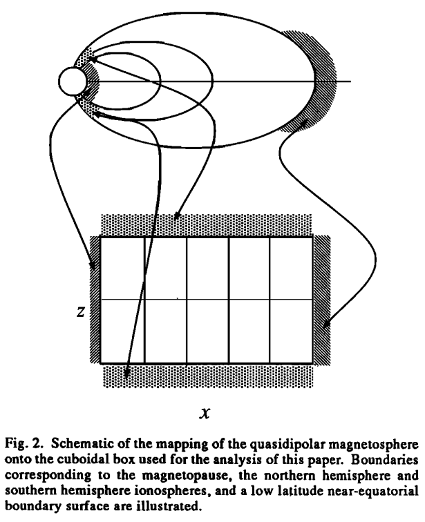
Southwood, 1974 proposed an elucidating 1D box model for field line resonance and later extended the model for various cases (e.g. Southwood & Kivelson, 1990). Instead of the actual dayside magnetosphere like a compressed dipole, we can simplify the geometry to something we can solve analytically. Imagine a field line with both footpoints connecting to the conducting ionosphere, we can map this curved field line into a straight line extending along z. In x direction, the outer boundary is the magnetopause, and the inner boundary is the reflection point. This is shown in the schematic figures below.

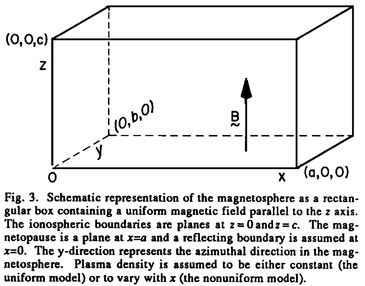
Plasma density $\rho_0$ varies only along the x-axis, while the background magnetic field is uniform and along the z-axis, i.e. $\mathbf{B}_0 = (0,0,B_0)$. Eliminating $\mathbf{B}_1$, $\mathbf{v}_1$ and $\mathbf{j}$ from Maxwell's equations lead to a wave equation for the linearized electric field perturbations of the form^[8]

$\frac{\partial^2\mathbf{E}}{\partial t^2} = \mathbf{V}_A\times\mathbf{V}_A\times\nabla\times(\nabla\times\mathbf{E})$

where the cross products are to be read from right to left, and $\mathbf{V}_A = \mathbf{B}_0 / \sqrt{\mu_0 \rho_0}$.

[8]	how to derive this? This is also different from Southwood's original derivation.

With the ansatz

$\mathbf{E}_\perp = (E_x(x), E_y(x), 0)\exp(ik_y y + ik_z z - i\omega t),$

and defining^[9]

[9]	I need to think about the unit of R: $1/m^2$?

$R^2(x) = \frac{\mu_0\rho_0(x)\omega^2}{B_0^2} = \frac{\omega^2}{V_A^2},$

the poloidal component (?) $E_y$ of the general wave equation is transformed into

$\frac{\partial^2}{\partial x^2}E_y - k_y^2 \frac{\partial}{\partial x}R^2(x)\frac{1}{(R^2 - k_z^2)(R^2 - k_z^2 - k_y^2)}\frac{\partial E_y}{\partial x} + (R^2 - k_z^2 - k_y^2)E_y = 0.$

This equation exhibits strong singularities found in the denominator of its $2^{nd}$ term, much as first described by Tamao (1965). The following solutions are possible. Let us first assume the case $R^2 - k_z^2 - k_y^2 > 0$, from which $R^2 - k_z^2 > 0$ follows. Thus, no singularities appear. Assuming further $k_y \approx 0$, the above equation reduces to

$\frac{\partial^2}{\partial x^2}E_y + (R^2 - k_z^2)E_y = 0.$

For a linear density profile, i.e. $R^2(x) = \alpha_0^2 + \alpha^2 x$, with the definition of the turning point $x_T$ via $R_T^2 = \alpha_0^2 + \alpha^2 x_T = k_z^2$, and the transformation $s = \alpha^{2/3}(x-x_T)$

$\frac{\partial^2}{\partial s^2}E_y + sE_y = 0.$

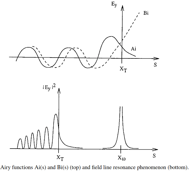
This is an Airy or Stokes differential equation^[10] with the two principal solutions displayed below. The solution $Bi(s)$ is unphysical as it implies unlimited growth of $E_y$ behind the turning point at $s=0$. Thus $E_y(s) = Ai(s)$ is the required solution. The turning point actually is the point of total reflection of the wave field. Its appearance can be understood on the following grounds. The fast mode dispersion relation is given by

$\frac{\omega^2}{k_x^2 + k_y^2 + k_z^2} = V_A^2,$

where $k_x$ is the wave number in the x-direction. If $V_A^2$ increases with x, that is with $s$ in the Airy function plot, $k_x^2$ has to decrease as $\omega, k_y$ and $k_z$ stay constant. Eventually $k_x^2$ may become negative, which implies an imaginary wave number $k_x$. At this turning point the wave will be reflected.

[10]	a good time to go back to Y.Y's note!

Considering the case $R^2 - k_z^2 - k_y^2 < 0$, $R^2 - k_z^2 = 0$ may occur. Assuming again a linear density profile, defining a resonance point $x_\omega$ via $R_\omega^2 = \alpha_0^2 + \alpha^2 x_\omega = k_z^2$, and $s = l(x-x_\omega)$, the electric field perturbation transforms close to the resonance point $x - x_\omega = 0$ into

$\frac{\partial^2}{\partial s^2}E_y + \frac{1}{s}\frac{\partial E_y}{\partial s} - E_y = 0,$

which is a modified Bessel equation. This is equivalent to Tamao's approach. At the resonance point its solution exhibits a clear singularity, that is unlimited growth of $E_y$. A discussion of the general solution of the electric field perturbation equation for the case $R^2 - k_z^2 - k_y^2 < 0$ is lengthy. Schematically the solution is given in the bottom panel of the above figure. It can be seen that in front of the turning point the solution is similar to an Airy function, while behind it singular behaviour is observed at the resonance point.

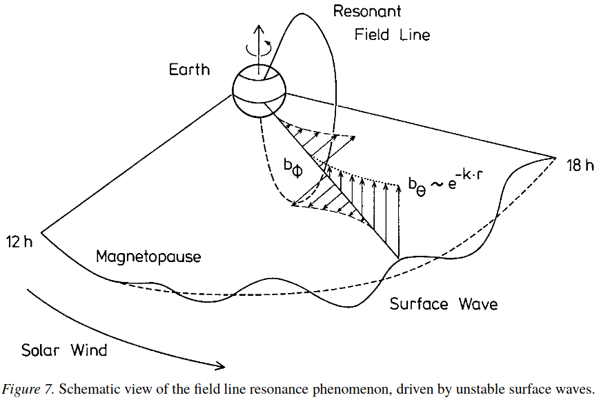
The following physical interpretation is tempting. The MHD wave propagating into the magnetosphere is a fast mode wave generated by, e.g., plasma instabilities at the magnetopause. Eventually the wave reaches the turning point where reflection occurs. If conditions are favourable, that is if a resonance point occurs, part of the fast mode wave energy can tunnel into the resonance, where coupling from the fast mode disturbance into an Alfvén mode perturbation takes place. This scenario is schematically shown in Figure 7, where the reflection or turning point is assumed to coincide with the magnetopause. The point of maximum coupling or “resonant mode coupling” is given by $\omega = k_\parallel V_A(x)$, where $\omega$ is the fast mode wave frequency, $k_\parallel$ is the field-aligned component of the fast mode wave vector and $V_A(x)$ is the local Alfvén velocity.

The energy that is carried into the magnetosphere across the background field by the non-guided fast mode is accumulated in the plane of resonant mode coupling (i.e., the y–z plane through $x_ω$ in the box model Figure) in the form of the guided Alfvén wave. It is this localized accumulation of energy due to resonant mode coupling between a non-guided mode and a guided mode that constitutes a field line resonance. This wave energy accumulation can be described by

$\frac{\partial w}{\partial t} + \nabla\cdot\mathbf{S} = -h,$

where $w$ is the wave energy density, $\mathbf{S}$ is the Poynting flux, and h a dissipation term, describing energy loss due to e.g. ionospheric Joule heating. As the background parameters only vary in the radial direction, this equation reduces to

$\frac{\partial w}{\partial t} = -\frac{d}{dr}S_x - h.$

Integration across the width of the coupling region in a radial direction leads to the following rate equation:

$\frac{\partial W}{\partial t} = c_e S_{ng} - S_h^{off} - H,$

where $W$ is the energy per area that is being accumulated in the coupling, $c_e$ is a coupling efficiency, $S_{ng}$ the incoming Poynting flux of the non-guided mode, and $S_g^{off}$ the “off-angle” component of the Poynting flux of that mode to which the non-guided mode couples. Including this term $S_g^{off}$ allows us to consider energy losses due to coupling to not strictly guided modes. A finite off-angle component of the coupled wave mode would render the energy accumulation less efficient or may even inhibit the build-up of a resonance. Off-angle components may arise if the transverse scale of the coupled wave become small enough for finite ion gyroradius or finite electron inertia becoming important. In this case the coupled mode is a kinetic Alfvén mode. The parameter $c_e$ denotes the coupling efficiency, that is the fraction of energy of the non-guided mode that is converted into the guided mode. Finally, H gives the dissipative losses, integrated in the x direction.

It is now instructive to evaluate the rate Equation for the ideal MHD regime. As the Alfvén mode is a strictly guided mode its Poynting flux is directed exactly parallel to the background magnetic field. In other words, $S_h^{off}=0$, and Equation reads

$\frac{\partial W}{\partial t} = c_e S_{fast},$

where $S_{fast} = S_{ng}$ is the Poynting flux of the non-guided MHD mode. Thus, the energy density in the coupling region is continuously increasing as there is no outward transport of energy to balance the incoming Poynting flux of the fast mode. However, ionospheric Joule heating provides a significant dissipation mechanism with H limiting the energy density.

Note that resonant mode coupling is only a necessary condition for field line resonances to occur. A sufficient condition is critical coupling to a strictly guided mode and absence of any dissipation.

At the resonance a phase shift of $180^o$ between the toroidal field components ($E_x$ in the box model, $b_\phi$ in the dipole coordinate) on both sides of the resonance is apparent. This phase shift can be understood using Maxwell's equations with the polarization current $\mathbf{j}_\perp = \rho_0/B_0^2\cdot d\mathbf{E}/dt$, and deriving

$(R^2 - k_z^2)E_x = ik_y \Big( \frac{\partial E_y}{\partial x} - ik_y E_x \Big) = k_y \omega b_z.$

At the resonance $R^2 = k_z^2$, thus $b_z=0$, and for the electric field polarization we have

$\frac{E_x}{E_y} = -\frac{i}{k_y E_y}\frac{\partial E_y}{\partial x}.$

The polarization therefore depends on $k_y$ as well as $\partial E_y/\partial x$. As $k_y$ changes sign across local noon for, e.g., K-H instability generated fast mode waves at the magnetopause and $\partial E_y/\partial x$ changes sign across the resonance point.

Let $\xi = (\xi_x, \xi_y, \xi_z)$ be the wave displacement vector and $B_{1z}$ be the compressional magnetic perturbation. Linearized MHD equations take the form

$\begin{aligned} \Big( \frac{\mu_0 \rho(x)}{B^2}\frac{\partial^2}{\partial t^2} + k_z^2 \Big) \xi_x &= -\frac{1}{B}\frac{\partial B_{1z}}{\partial x} \\ \Big( \frac{\mu_0 \rho(x)}{B^2}\frac{\partial^2}{\partial t^2} + k_z^2 \Big) \xi_y &= -ik_y\frac{B_{1z}}{B} \\ b_z = -ik_y B \xi_y - B\frac{\partial \xi_x}{\partial x} \end{aligned}$

First assume we have uniform B field $\mathbf{B} = B_0 \hat{z}$ but a 1D density variation $\rho = \rho(x)$. This will give us a changing Alfvén speed as a function of x. We are looking for solutions $\sim B_{1z}(x)e^{i(\omega t - k_y y)}\cos(k_z z)$ (i.e. purely standing wave along the magnetic field lines or in the poloidal direction, wave+damp/growth along y or in the toroidal direction). From the linearized MHD equations, what we end up with is a 2nd order differential equation

$\frac{d^2 B_{1z}}{dx^2} - \frac{\omega^2 V_A^2 \frac{d V_A^2}{dx}}{\omega^2 - \omega_A(x)^2}\frac{d B_{1z}}{dx} + \Big( \frac{\omega^2}{V_A^2} - k_y^2 - k_z^2 \Big) B_{1z} = 0$

Several observations from this equation:

1. Singular point at $\omega = \omega_A$: Alfvén resonance.

2. Turning point at $\frac{\omega^2}{V_A^2} - k_y^2 - k_z^2 = 0$: effectively $k_x = 0$ (???)

Later simulations confirm the coupling between fast and Alfvén mode based on this model. The initial energy injection through fast mode can be converted to Alfvén mode energy and lead to energy density increase at certain locations with certain frequencies.

Secondly, Consider, therefore, a cold plasma contained in a volume of sides a, b, c, in which the density $\rho$ and the field $B \mathbf{e}_z$ are uniform. We are interested in the response of this system to a pressure variation of the form

$\exp (ik_y y + ik_z z) p(t)$

imposed at the boundary, x = a. As pressure balance is maintained across the boundary, there will be a magnetic compression in the cold plasma inside the boundary with a corresponding field perturbation $b_z(t)$ at x = a.

Inside the plasma cavity the compressional field perturbation can be written

$b_z(x, t) \exp(ik_y y + ik_z z)$

where $k_y$ and $k_z$ are arbitrary. The perturbation, bz(x,t), obeys the MHD equations

...

Possible solutions (essentially analytical form of $b_z$ perturbation):

1. compression and motion directly in phase with the boundary perturbation

2. compression and motion in antiphase with the boundary perturbation

3. transverse oscillations (Alfvén mode)

4. cavity modes of the fast MHD mode

5. some combination of the above.

What occurs in any given situation depends on the frequency spectrum of the source.

More details shall be found in Theory of hydromagnetic waves in the magnetosphere and Southwood & Kivelson, 1990.

Limitations of Current FLR theory

The mathematical description of field line resonance (FLR) often assume a simple dipole magnetic field which is not appropriate to high latitudes where field lines experience significant temporal distortion. This affects the frequency and polarization properties of the FLRs. The latter is important because wave-particle energy transfer involves the wave electric field component parallel to the drift velocity of particle, i.e. the azimuthal field (poloidal mode) in a dipolar magnetic field.

The Poynting flux is field aligned and away from the equatorial plane. These waves likely arise from incoming compressional mode

Simply speaking, the nice math derivations does not work for nonideal magnetic field setup. Observers are clueless in knowing what is really going on.

The MHD wave equations that describe the coupling between the fast compressional mode and the shear Alfvén mode are complicated and have not been completely solved analytically, even in a simple dipole geometry.

All mode identifications are based on linearized theory in a homogeneous plasma and there are clear indications, in both the data and in numerical simulations, that nonlinearity and/or inhomogeneity modify even the most basic aspects of some modes. For example, in the nonuniform case the ULF waves can couple.

Turbulence is also frequently observed in the magnetosheath, i.e. O(1) fluctuations in density, bulk velocity, and magnetic field over a broad range of frequencies. Classical theories generally do not consider turbulence.

Types of Variations

Alfvénic

Rotational Discontinuity

Simulations

Korean MHD Model

spherical, $10 \text{R}_E$ < r < $40 \text{R}_E$, $10^o < \theta < 170^o$, $0^o < \phi < 180^o$.^[11]

[11]	For bow shock and sheath study, this might be good enough since it's super-Alfvénic and super-sonic.

$n = 5$ amu/cc, $B_0 = 10$ nT with $45^o$ from the x axis (in the x-y plane, Parker-spiral like), $T = 10^6$ K, $V = (-500,0,0)$ km/s, which turns to $M_A \sim 5$, $V_A \sim 100$ km/s, $\beta \sim 1.7$.

3 types of density pulses:

• density variation only, everything else constant

$\delta \rho = \rho_0 sin(\omega t) \text{for } 0 \le t \le T/2$

where $T = 2\pi/\omega \sim 100s$. Note that this perturbation is relatively large (max 100%).

• fast/slow mode

$\begin{aligned} \delta \rho = \rho_0 sin(\omega t) \\ \delta p = C_s^2 \delta\rho \\ \delta B_x = \delta B_z = 0, \delta B_y = \pm B_{y0}\delta \rho/\rho_0 \end{aligned}$

where $C_s$ is the sound speed in the solar wind and the $+/-$ sign refers to the fast/slow type perturbation.

• density only, but stronger peak

$\delta \rho = 4\rho_0 exp[-(t-t_c)^8]$

where $t_c$ is just an arbitrarily chosen parameter.

Interaction outcomes: fast mode –> shock, slow mode, entropy wave.

[Lee+, 2008]full wave equations for a cold plasma

LFM

nonlinear TVD scheme switches to allow shock capturing

Boris correction is applied to the perpendicular component of the displacement current in the $\mathbf{J}\times\mathbf{B}$ force of the MHD momentum equation, but with an artifically low speed of light.

Single-fluid, ideal MHD, $\sim 0.25\, \text{R}_E$ resolution in the inner magnetosphere, upstream boundary at $x=30\, \text{R}_E$ in GSM coordinates. Fixed upstream solar wind condition ($B_x$, $V_x$), outflow on all other sides. They introduce an out-of-phase oscillation in the input sound speed time series (~ 40 km/s), so as to hold the thermal pressure constant in the upstream solar wind ($p_{th} \propto nC_S^2$). I don't quite understand this technique.

Inner boundary: 2D electrostatic model of the ionosphere, with electric potential obtained from Poisson's equation and then mapped along the dipole field lines back to the inner boundary of MHD at about $2\, \text{R}_E$. The ionospheric conductance, needed for the potential solver, is specified by an empirical extreme ultra-violet (EUV) conductance model and by a contribution from particle precipitation.

When starting the runs, they choose to flip the IMF direction multiple times which they call "precondition". Reason? Faster? Higher accuracy? Stability?

LFM model by Claudepierre+, 2008: The phase velocities of the modes were different but the frequencies were the same and depended on the solar wind driving velocity. For both modes the preferred wavenumber was related to the boundary thickness, so that the K-H waves are monochromatic.

In Claudepierre+, 2009, LFM is used to study the magnetospheric response to only a fluctuating upstream dynamic pressure. The changing of dynamic pressure is done through changing number density while keeping bulk velocity constant. The input dynamic pressure has frequency components spreading across Pc3 to Pc5 ranges:

Frequency (mHz)	Relative Oscillation Amplitude (%)
5	20
10	20
18	30
25	40[12]
0-50	20

Background $\rho = 5$ amu/cc, $B = (0, 0, -5)$ nT, and $V = (-600, 0, 0)$ km/s. In Figure 1, the authors demonstrate the filtering/attenuation of the higher frequency spectral components, which is an expected artifact of the numeric solver, unfortunately. I haven't checked the shift or attenuation of frequency in Vlasiator (numerical Vlasov solver), but obviously the amplitude decreases.

Results:

1. Strong peak signal observed around 10 mHz in the continuum band input run.

2. PSD of $B_z$, $E_\phi$, the two compressional components of EM fields along the noon-meridional line, shows strong $B_z$ signals near the magnetopause.

3. They argue that the outputs represent MHD cavity modes, which in the simplest interpretation, can be thought of as standing waves in the electric and magnetic fields between a cavity inner and outer boundary. [Kivelson and Southwood, 1985]

The cavity frequency in a simple box geometry configuration with perfect conductor boundary conditions:

$f_n = \frac{V_A}{2a}n,\, \text{for} n = 1,2,3,...$

where a is the box length in x direction.

In Claudepierre+, 2010, they show that the monochromatic solar wind dynamic pressure fluctuations drive toroidal mode field line resonances (FLRs) on the dayside at locations wherethe upstream driving frequency matches a local field line eigenfrequency.

Frequency (mHz)	Relative Oscillation Amplitude (%)
10	20
15	20
25	40[13]
0-50	20

[13]	The larger oscillation amplitude for the input time series in the 25 mHz simulation is used to combat the effects of anumerical attenuation/filtering of higher‐frequency compo-nents in the LFM simulation.

In Figure 2 of this paper, you can clearly see the attentuation in shorter wavelengths beyond 15 mHz after propagating for 10 $\text{R}_E$.

A useful quantity called root-integrated power (RIP) for a given time series:

$RIP = [\int_{f_a}^{f_b}P(f) df]^{1/2}$

where $P(f)$ is the power spectral density of the given time series and the integration is carried out over a given frequency band of interest, $[f_a, f_b]$.

In this paper, the RIPs are calculated for $E_r$ and $B_\phi$ under the cyclindrical polar coordinates (which I believe are the two compressional components?).

From Alfvén speed profiles, we can compute estimates to the natural oscillation frequency for a given field line. For example, the WKB estimate to the field line eigenfrequency is given by [Radoski, 1966]^[14]

$f_n = n[2\int_S^N \frac{ds}{v_A(s)}]^{-1} \, \text{for } n=1,2,3,...$

where n is the harmonic number of the FLR, s is the arc length along the field line, and the integration is carried out from the southern field line foot point (S) to the northern foot point (N). This estimate to the field line eigenfrequency is essentially the inverse of the travel time for an Alfvén wave propagating along the magnetic field line to bounce off the reflecting ionospheres and return to its starting point. It is a good approximation for the higher harmonics (large n) and predicts a value about 20% higher than the actual fundamental mode. The factor of 2 in the above equation is due to the a forementioned "bouncing" and due to the perfectly conducting ionospheric boundary condition assumed in FLR theory.

[14]	This WKB approximation assumes dipole field, but the real magnetic field is compressed on the dayside.

Figure 3 is the most important and informative plot. In order to reproduce this kind of plot, I need:

• field tracer

• density and magnetic field along the traced field line

• conversion from Cartesian to spherical coordinates

• outputs from a time series^[15]

[15]

In order to obtain PSD, the total simulation time shall be much larger than the enforced frequency. In MHD simulations which are relatively cheap, it is quite easy to run for hours and look at PSD of frequency in the Pc3-5 range. For Vlasov simulation, even in 2D, up until now (2021/08/16) I only have ~300s, which is only 2 periods of the enforced perturbation in density.

In later sections there are additional discussions about polarization and energy flux (Poynting vector), but those are minor details.

###

Wright and Allan, 2008: numerical simulations of MHD wave coupling in the magnetotail waveguide that suggested 5–20 min fast mode waves generated in the magnetotail waveguide by substorms may couple to Earthward propagating Alfvén waves and produce field-aligned currents resulting in narrow auroral arcs that move equatorward at ∼1 km/s.

self-written model with no name

###

Jordanova+, 2007 used a global ring current-atmosphere interactions model (RAM) including a time-dependent plasmasphere to determine the EMIC growth rate with time.

###

Ray tracing calculations by Chen et al. (2009) of ICW growth

###

McCollough et al. (2009) using a 3-D test particle solver coupled to the time-dependent MHD fields produced by the global LFM code.

###

Test-particle simulations have shown that perturbations in electric and magnetic fields are induced across wide regions of the magnetosphere by global magnetospheric compressions due to ULF variations in solar wind dynamic pressure and presumably also FLRs and magnetosonic waves (Ukhorskiy et al. 2006).

Techniques

MHD Waves Detection

ULF waves are MHD waves: Alfvén wave, fast wave and slow wave. One basic approach to identify waves is to check the correlation of quantity perturbations.

The phase speed of shear Alfvén wave is

$v_{pA} = \frac{\omega}{k} = v_A \cos{\theta}$

where $v_A$ is the Alfvén speed and $\theta$ is the angle between wave vector $\mathbf{k}$ and magnetic field $\mathbf{B}$.

The perturbed quantities of Alfvén waves follow the relations

$\begin{aligned} \frac{\delta \mathbf{v}}{v_A} &= \pm \frac{\delta \mathbf{B}}{B_0}, \\ \delta \rho &= 0, \end{aligned}$

where $\delta \mathbf{v}$, $\delta \mathbf{B}$, and $\delta \rho$ are perturbed plasma velocity, magnetic fields, and plasma density, respectively, and $B_0$ is the background magnetic magnitude.

For slow and fast waves, the phase speeds are

$v_{p\pm}^2 = \big(\frac{\omega}{k} \big) = \frac{1}{2}(V_s^2 + V_A^2) \pm \frac{1}{2}\Big[ (V_s^2 + V_A^2)^2 - 4V_s^2 V_A^2 \cos^2{\theta}\Big]^{1/2}$

The "+" is for fast waves and "−" for slow waves, and $V_S$ is the sound speed. The perturbed quantities for fast and slow waves are

$\begin{aligned} \delta \rho &= \frac{\rho_0}{v_p}\frac{v_A^2\sin\theta}{B_0 (v_p - v_s^2/v_p)}\delta B, \\ \delta \mathbf{v} &= -\frac{v_A^2 \cos{\theta}}{B_0 v_p}\delta\mathbf{B} + \frac{v_A^2 \sin{\theta}\delta B}{B_0 (v_p - v_s^2/v_p)}\frac{\mathbf{k}}{k}. \end{aligned}$

Thus generally the Alfvén wave is identified by the correlations between velocity and magnetic field perturbations, and the fast and slow waves are identified by the negative (for slow waves) or positive (for fast waves) correlations between either density and magnetic field perturbation or thermal pressure and magnetic pressure perturbation.

The second equation above can also be expressed in terms of magnetic and thermal pressure pertubations

$\delta P_B = \frac{\mathbf{B}_0 \cdot \mathbf{B}}{\mu_0} = \frac{V_A^2}{V_S^2}\left(1-\frac{k^2 V_S^{2} \cos^2\theta}{\omega^2}\right)\delta P_t$

See the lecture notes for more details.

For the magnetosonic waves, consider using $\delta \mathbf{E}$ and $\delta \mathbf{B}$ for identifying speed. The slopes of the curves $\delta E∕\delta B$ correspond to the wave propagation speed in the spacecraft frame.

Transverse and shear Alfvén wave refer to actually the same thing: the descriptions arise from $\mathbf{k}\cdot\mathbf{V} = 0$ and $\mathbf{V}\cdot\mathbf{B}_0 = 0$.

The fast and slow magnetosonic waves are associated with non-zero perturbations in the plasma density and pressure, and also involve plasma motion parallel, as well as perpendicular, to the magnetic field. The latter observation suggests that the dispersion relations $\omega = kV_{\pm}$ are likely to undergo significant modification in collisionless plasmas. In order to better understand the nature of the fast and slow waves, let us consider the cold-plasma limit, which is obtained by letting the sound speed $V_S$ tend to zero. In this limit, the slow wave ceases to exist (in fact, its phase velocity tends to zero) whereas the dispersion relation for the fast wave reduces to

$\omega = kV_A.$

This can be identified as the dispersion relation for the compressional-Alfvén wave. Thus, we can identify the fast wave as the compressional-Alfvén wave modified by a non-zero plasma pressure.

In the limit $V_A\gg V_S$, which is appropriate to low-β plasmas, the dispersion relation for the slow wave reduces to

$\omega \simeq k\,V_S\,\cos\theta.$

This is actually the dispersion relation of a sound wave propagating along magnetic field-lines. Thus, in low-β plasmas the slow wave is a sound wave modified by the presence of the magnetic field.

In reality, waves can be mixed together with mode conversions. Also, notice that the classical wave theory is based on spatially homogeneous plasma assumption, which is rarely the case in nature such as the magnetosphere.

A tricky part in practice is how to get the average through smoothing. Note that a real satellite moves both in time and space. Usually people do moving-box-average to get an average state within a short period.

A more careful analysis is called Walén test.

However, always keep in mind that the most reliable way of identifying waves is to calculate the dispersion relation.

Polarization analysis

Singular Value Decomposition (SVD): Lee & Angelopoulos

hodogram of field components

Wave vector direction

The direction of the wave vector can be estimated using MVA on the measured magnetic field. For plane waves, the propagation vector lies along the minimum variance direction.

Phase coherent technique

It is used to check the relation of one frequency oscillation to another.

Fourier transform

It can be used for

• determining the energy spectrum density for waves in a certain range

• automated ULF wave detection algorithms.

Wavelet transform technique

Wavelet Transform decomposes a function into a set of wavelets. A Wavelet is a wave-like oscillation that is localized in time. Two basic properties of a wavelet are scale and location.

Key advantages of Wavelet Transform compared with Fourier Tranform:

• Wavelet transform can extract local spectral and temporal information simultaneously, while FT only extract global information.

• There are various wavelets to choose from. In practice, if you have any prior knowledge to the signal you want to identify, you can find for an appropriate wavelet that is close to that shape.

A nice introduction can be found here. A practical example of R Wave Detection in the ECG using wavelet transform is given in Matlab.

For example, Morlet/Gabor wavelet is a wavelet composed of a complext exponential (carrier) multiplied by a Gaussian window (envelope).

Superposed epoch analysis

A statistical tool to detect periodicities within a time sequence or to reveal a correlation in time between two time series.

1. Define each occurrence of an event in one data sequence as a key time.

2. Extract subsets of data from the other sequence within some time range near each key time.

3. Superpose all extracted subsets from series 2.

An example of sunspot analysis can be found here. This sounds easy, or even too easy. I won't even consider it a standard method...