Overview of Ganymede's Simulations
resistive MHD
The simulation domain is \(10 R_G\) surrounding Ganymede. Outer boundary may have reflections that effect the inner solution, and the inner BC \(\mathbf{v}=0\) is inconsistent with the flow measurements from Galileo Plasma Subsystem (PLS).
The BCs are not clearly mentioned.
Multifluid MHD
Paty+, 2004, Paty+, 2006, Paty+, 2008
The inner boundary lies along the base of the ionosphere, which is held constant on the assumption of a constant source of ionospheric and exospheric material from surface sputtering. Plasma incident on this boundary is lost to the simulation since neither the chemical effects associated with generation of aurora or the surface sputtering is included in the model.
| Variables | Inner Boundary | Outer Boundary (upstream) |
|---|---|---|
| \(\rho\) | fixed, \(H^+\) 2000 \(\text{cc}^{-1}\), \(O^+\) 1000 \(\text{cc}^{-1}\) | fixed, 30 amu/cc |
| \(P\) | scale height \(H=263\) km, 9.0 to 0.1 eV from polar to equatorial | fixed |
| \(\mathbf{V}\) | float | fixed, 180 km/s |
| \(\mathbf{B}\) | ? | fixed |
They want to incorporate the effect of multiple ion species. However, the model has some issues with the configuration of the magnetosphere, such that the magnetic field comparison is not good.
Single fluid MHD, 2008-2010
4 Eqs. stretched spherical coordinates, leapfrog time marching, central differencing in space.
To maintain \(\nabla\cdot\mathbf{B}=0\) condition, the magnetic potential \(\mathbf{A}\) is used instead of magnetic field \(\mathbf{B}\).
Semi-implicit method: introduces a term into the momentum equation that effectively modifies the inertial of the short-wavelength modes, while accurately treating the long wavelengths, enabling the timestep to exceed CFL limit for Alfvén and magnetosonic waves. It achieves efficiency by removing short-wavelength high-frequency oscillations, which are on the scale of grid spacing. Preconditioned conjugate gradient method is used to invert the matrices.
\(r \in [0.5,40] R_G\), \(131\times 132\times 128 (r,\theta,\varphi)\) grid points. finest grid resolution in \(\widehat{r}\sim 0.01 R_G \approx 26\text{km}\), average within the magnetosphere \(0.04 R_G\approx 100\text{km}\).
The best BCs being advertised:
| Variables | Core Boundary (\(r=0.5R_G\)) | Surface Boundary (\(r=1R_G\)) | Outer Boundary (upstream) | Outer Boundary (downstream) |
|---|---|---|---|---|
| \(\rho\) | fixed, \(550 \text{amu}/cm^3\) | fixed | float | |
| \(P\) | fixed, \(0.125\textnormal{nPa}\) | fixed | float | |
| \(\mathbf{V}\) | \(\mathbf{V}\perp\mathbf{B}\) | fixed | float | |
| \(\mathbf{B}\) | dipole | fixed | float |
The pressure and density at the surface boundary corresponds to an average temperature of 20 eV
Core BC
Set tangential \(\mathbf{E}\) to be 0 (I don't know what this means and why.)
Advance the magnetic field between inner BC and core BC by setting \(\mathbf{v}=0\)[1], so that there are only magnetic diffusion and numerical diffusion. make the diffusion time very long compared to the typical Alfvén timescale by adjusting \(\eta\). \(v_A=220\text{km/s}\), Lundquist number \(\sim 4000\)[2].
| [1] | My guess is that the implementation is similar to the initial Mercury user module in BATSRUS. This magically works, but violates the basic principles of CFD. |
| [2] | In plasma physics, the Lundquist number (denoted by S) is a dimensionless ratio which compares the timescale of an Alfvén wave crossing to the timescale of resistive diffusion. It is a special case of the Magnetic Reynolds number when the Alfvén velocity is the typical velocity scale of the system, and is given by \[ S=\frac{Lv_A}{\eta} \] where \(L\) is the typical length scale of the system, \(\eta\) is the magnetic diffusivity and \(v_A\) is the Alfvén velocity. High Lundquist numbers indicate highly conducting plasmas, while low Lundquist numbers indicate more resistive plasmas. Laboratory plasma experiments typically have Lundquist numbers between \(10^2-10^8\), while in astrophysical situations the Lundquist number can be greater than \(10^{20}\). Considerations of Lundquist number are especially important in magnetic reconnection. |
Inner BC
\(r=1.05R_G\), ionosphere is treated as a finite-conductivity thin layer populated with cold dense plasma. uniform plasma density and pressure,
\[ n_{surf}=550\text{amu/cm}^3,\ n=39\text{cm}^3 \] \[\begin{aligned} T_{surf} = 20eV=20/(1.38\times10^{-23})\cdot 1.6\times10^{-19}=2.32\times10^5K, \\ P_{surf}=nk_B T=39\cdot 10^{6}\times k_B\times 20/k_B \cdot(1.6\cdot 10^{-19})\text{Pa}=0.125\text{nPa} . \end{aligned}\]Flows stop at this BC, \(\mathbf{v}=0\). \(\eta\) in this layer increases from the background value used far from Ganymede (nearly \(0\), which means fully conducting) to the value assumed at the surface in order to mimic the finite electric conductance of the ionosphere. uncertain ionosphere conductance, height-integrated conductance \(\Sigma=2S\) in the setup.
Later Duling+, 2014 questioned this approximation. The extension of the resistivity profile outside the surface is only a numerical consideration, which is probably incorrect.
Forcing the ionospheric flow to be zero is a reasonably good approximation for a highly conducting obstacle. However, the moon's mantle is most likely to be quite weakly conducting and the conductance of Ganymede's ionosphere is quite uncertain.
Ionosphere can be considered as a reservoir populated with cold and dense plasma. \(\rightarrow\) constant plasma density and pressure is applicable. (From CFD perspective, fixing both density and pressure is overspecification.)
reflect \(U\): \(\mathbf{v}_r=0,\mathbf{v}_\theta\) and \(\mathbf{v}_\phi\) continuous.\(\rightarrow\) float. This allows the boundary to act as a hard wall with respect to the flow and prevents the plasma from penetrating the boundary. However, not allowing the flow go through the boundary is not appropriate for an ionosphere with finite conductance.
\(B\) dependent \(U\): requires the component of the flow velocty perpendicular to the local magnetic field to be continuous at the inner boundary, \(\mathbf{v}_{\perp1}=\mathbf{v}_{\perp2}\), where \(\mathbf{v}_\perp=\mathbf{v}-\frac{\mathbf{v}\cdot\mathbf{B}}{B}\widehat{b}\)
Resistivity profile: between the core boundary \(r=0.5R_G\) and the moon's surface \(r=1.0R_G\) is the insulating rocky mantle whose electrical conductivity is extremely low (\(\sim 0\)). No plasma flowing in this region, the model solves for a magnetic diffusion equation only. High numerical resistivity corresponding to a Lundquist number of \(0.2\) in this region.
The flowing plasma outside the ionosphere (\(r>1.05R_G\)) is regarded infinitely conducting \(\eta=0\). In terms of conductivity, the ionosphere, whose finite conductivity arises from neutral-ion collisions, can be considered as a transition layer between the insulating mantle and the highly conducting magnetosphere. In the setup, we let the ionospheric resistivity decrease monotonically from its value in the mantle to its background value outside the ionosphere.
\[ \eta=\eta(r) \]An anomolous resistivity being setup to enable fast reconnection to occur in regions where magnetic shear is strong. It is introduced only outside the ionosphere and is turned on only at locations where the local current density exceeds some threshold.
Outer BC
\(r=20 R_G\), divided into upstream (\(X\le 0\)) and downstream (\(X>0\)). Fix \(\rho,P,\mathbf{v},\mathbf{B},\mathbf{E}_t\) on all points at the upstream; non-reflecting BC, free-to-leave (float) at the downstream. The flow speed in the reference frame of Ganymede is
\[ \mathbf{v}=140 \text{km/s} \]The average plasma \(n\) is around \(4\text{ cm}^{-3}\) with a range from \(1\) to \(10\text{ cm}^{-3}\). Assuming that mass-charge ratio is \(14\), and ions are singly charged. For G8 pass,
\[ P_t=3.8\text{nPa} \]so that the Jovian wind temperature is
\[ T_{solar} = P/(nk_B)=3.8\text{ nPa}/(4\times 10^{6}*1.38\times10^{-23})/1.2=5.7367\times10^7 K \]This is equivalent to about \(6000eV\). The coefficient \(1.2\) corresponds to the original settings of ion/electron temperature ratio \(5\).
This large temperature results from the simplification of single fluid MHD. In Table 21.1 of [Kivelson+, 2004][Kivelson+2004], the average ion temperature around the equator is about 60 eV and the average electron temperature is about 300 eV. With an average ion number density of 4, this gives a thermal pressure of only 0.04 nPa. However, there are also a significant contributions to the pressure from energetic ions (20 keV - 100 MeV ions) of 3.6 nPa and hot electrons of 0.2 nPa, which in total gives 3.8 nPa pressure. In order to compensate for the missing energetic species from the single fluid MHD simulation, we have to prescribe a much hotter plasma.
The initial model in 2008 without resistivity generates a magnetopause which is \(10\%\) smaller than the observed one for G28.
The later improved model in 2009 tunes the resistivity.
The Dungey-cycle like global flow pattern should be: plasma flow is brought into the magnetosphere mainly through reconnection on the upstream side and in turn convects over the polar cap into the downstream region. Then it is expected to partially return toward the moon and upstream at low latitude (\(z=0\) cut).
Ideal MHD with Non-Conducting Surface
| Variables | Inner Boundary | Outer Boundary (upstream) | Outer Boundary (downstream) |
|---|---|---|---|
| \(\rho\) | float | fixed | float |
| \(e\) | float | fixed | float |
| \(\mathbf{V}\) | absorb | fixed | float |
| \(\mathbf{B}\) | insulating | fixed | float |
The magnetic insulating BC is complicated. Even until now I don't fully understand the derivation.
They didn't show any plots or had any comments related to pressure nor temperature. This probably means that they only considered the thermal component of the plasma, similar to what Fatemi+, 2018 did.
Atmosphere and ionosphere
Four factors are considered:
ion‐neutral collision in the atmosphere
ionization due to solar radiation
recombination
magnetic diffusion (refer to the original paper)
For the atmosphere they assume \(O_2\) with radially symmetric distribution and 0 initial velocity. When plasma particles collide with the neutral molecules, the plasma loses momentum. The amount of momentum loss is modeled through a collision frequency on the RHS of the momentum equation,
\[ - \nu_n \mathbf{V}, \] \[ \nu_n(r) = \sigma_n V_0 n_n(r) \]which is a function of the \(O_2\) cross section \(\sigma_n = 2.0\times10^{-19}\,m^2\), typical plasma flow velocity \(V_0\), and the number density of \(O_2\) molecules in the atmosphere.[3] Nevertheless, the collision frequency is only a weak function of \(V\) since \(\sigma_n\) scales approximately with \(V^{-1}\) for elastic collisions in the polarization approximation.
| [3] | Note that ion-neutral collisions occur predominantly near the surface where the plasma flow speed \(V\) is significantly reduced from the Jovian background flow speed \(V_0\). That's why there's no velocity difference in the formula. |
They choose a scale height \(H = 250\) km even though the real scale height close to the surface is likely smaller. With an estimated column density \(N_n = 2\times10^{14} \text{cm}^{−2}\)[4] and the chosen scale height, the estimated number density on the surface is about \(n_{n,0} = N_n∕H \approx 8.0\times10^{12} \text{m}^{−3}\).
| [4] | A later paper argued that a 10 times larger column density is required to reproduce the correct electron number density during the G2 flyby close encounter. |
This process is characterized by a production rate
\[ P(r) = \nu_{\text{ion}}n_n(r). \]For simplicity a globally averaged and constant solar radiation is assumed and the shadow caused by Ganymede’s body as well as the variability of Ganymede’s position on its orbit are neglected. Therefore, the production rate directly scales with the density of the atmosphere and thus only has a radial dependency. The photo-ionization rate is chosen to be \(\nu_\text{ion} = 2.2\times10^{−8} \text{s}^{−1}\).
Because plasma consists of molecular ions and electrons, it can be lost through dissociative recombination. The occurrence of recombination depends on the thermal energy of the electrons and consequently the recombination rate is a function of the plasma particle density \(n = \rho∕m_i\) and the electron temperature \(T_e\). An empirical dissociative recombination rate coefficient is applied
\[ \alpha = 1.6 \Big(\frac{300\,\text{K}}{T_e}\Big)^{0.55}\times 10^{-13} \text{m}^3/\text{s} \]of gaseous oxygen for temperatures higher than 1200 K. An electron temperature of \(k_B T_e = 0.1\,\text{eV}\approx 1160\,\text{K}\) is used and results in \(\alpha \approx 7.8\times10^{-14}\,\text{m}^3/\text{s} \). Since the real electron temperature is unknown, whichever yields a reasonable ionospheric mass density is chosen. To avoid the ion plasma density decreases below the mostly atomic background ion density \(n_0 = \rho_0∕m_i\), the loss rate is modified by
\[ L(\mathbf{r},t) = \begin{cases} \alpha n(\mathbf{r},t)(n(\mathbf{r},t) - n_0) & \text{for } n(\mathbf{r},t) > n_0,\\ 0 & \text{for } n(\mathbf{r},t) \le n_0. \end{cases} \]When equalizing the production and loss rate to receive the plasma number density at the surface in chemical equilibrium,
\[ n_s = \sqrt{\frac{\nu_\text{ion}n_{n,0}}{\alpha}}. \]The estimated surface density the therefore around \(n_s\approx 1500\, \text{cm}^{-3}\), which is higher than previous observation and close to another model estimation.
In order to achieve this equilibrium, they ran the model for approximately 1.2 million iterations with a time step controlled by the Courant‐Friedrichs‐Lewy criterion which respects all physical effects.
One thing worth noticing here is that in the final simulation result, the peak density is about 2350 [\(\text{amu}/\text{cc}\)], or 75 [\(\text{cc}^{-1}\)], which is 20 time smaller than the estimated value above. They claimed that it is because the convection term partly balances the source term instead.
Aurora Estimation, 2015
Payan
MHD-EPIC
| Variables | Inner Boundary | Outer Boundary (upstream, downstream) | Outer Boundary (sides) |
|---|---|---|---|
| \(\rho\) | float | fixed | float |
| \(P\) | float | fixed | float |
| \(\mathbf{V}\) | absorb | fixed | float |
| \(\mathbf{B}\) | float for \(\mathbf{B}_{1\theta}\) and \(\mathbf{B}_{1\phi}\), reflect for \(\mathbf{B}_{1r}\) | fixed | float |
\([-128,128]R_G\), smallest cell size is \(1/32R_G\) in a box \(x\in [-3,4],y\in [-3,3], z\in[-2,2]\) total 8.5 million cells.
simple fixed inflow and zero-gradient outflow BCs (typically used for the solar wind around planetary magnetospheres)do not work for the subsonic and sub-Alfv\'{e}nic Jovian wind.
Hall effect region: \(|x|<4R_G,\ |y|<3 R_G,\ |z|<2R_G\) box.
The flows shown in Fig.5 in \(z=0\) cut is very strange. This is Hall MHD results.
The standoff distance is 6% larger than observation.
Hybrid Model
Ions treated as fully kinetic particles:
\[ \frac{d\mathbf{u}}{dt} = \mathbf{E} + \mathbf{u}\times\mathbf{B} -\nu (\mathbf{u}_i - \mathbf{u}_e) \]Electrons treated as massless fluid: (?)
\[ \mathbf{u}_e = \mathbf{u}_i - \frac{\nabla\times\mathbf{B}}{\alpha N} \]The electric field is calculated from the electron momentum equation:
\[ \mathbf{E} = -\mathbf{u}_e\times\mathbf{B} - \frac{\nabla \tensor{P}_e}{N} -\nu(\mathbf{u}_e - \mathbf{u}_i) \]The magnetic field advanced in time using Faraday's law:
\[ \frac{\partial\mathbf{B}}{\partial t} = -\nabla\times\mathbf{E} \]Parallel hybrid multi-grid model
The incident plasma is injected at the entry plane following a Maxwellian velocity distribution.
Particle BC:
periodic boundary conditions are used to deal with particles coming from the incident plasma flow;
planetary particles are lost when leaving the simulation domain.
The BCs are not fully described in the paper.
| Variables | Surface Boundary (\(r=1R_G\)) | Outer Boundary (upstream) | Outer Boundary (downstream) | Outer Boundary (side) |
|---|---|---|---|---|
| Particle | fixed, 0 | Maxwellian | float | particle-dependent |
| \(\mathbf{E}\) | ? | fixed, \(-\mathbf{V}\times\mathbf{B}\) | float | periodic |
| \(\mathbf{B}\) | ? | fixed | float | periodic |
Outer boundary condition: \(T_i = T_e = 200\,\text{eV}\), \(n_i = 4\,\ text{cm}^{-3}\). The author claims that using a slightly higher than average (60 eV) temperature would compensate the missing of energetic particles, but this is obviously impossible. To get the 3.8 nPa upstream pressure with the given \(n_i\), the average temperature would be as high as 6000 eV. This won't make much of a difference to the magnetopause location because the pressure balance is predominantly determined by the magnetic pressure and dynamic pressure.
They do not specify the inner boundary conditions in the published paper. While they have kinetic ions in their model, only the simulated electric and magnetic fields are used in another test particle model to compute the precipitation fluxes for the energetic particles. This probably means that there are some issues with the hybrid model itself, otherwise why not use the information from the model directly?
Wang, 2018
10-moment equation model.
Exosphere
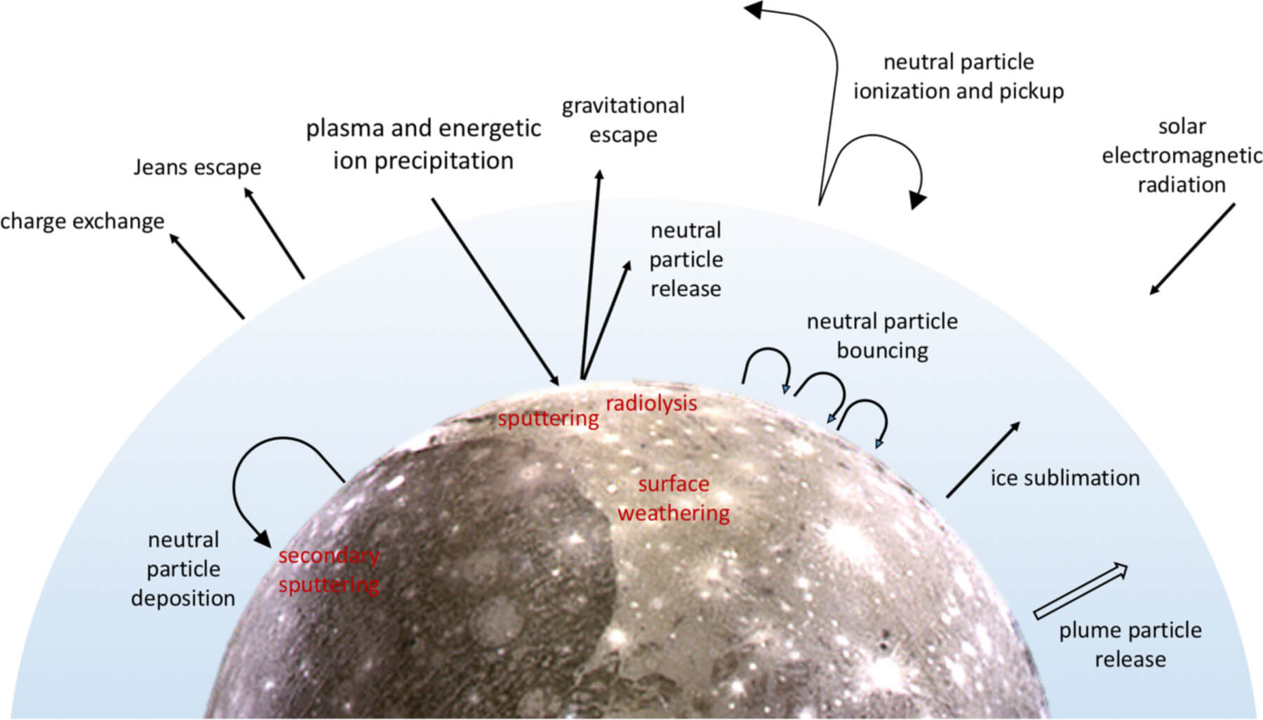 Possible source and loss mechanisms for the exosphere of Ganymede.
Ionosphere Model
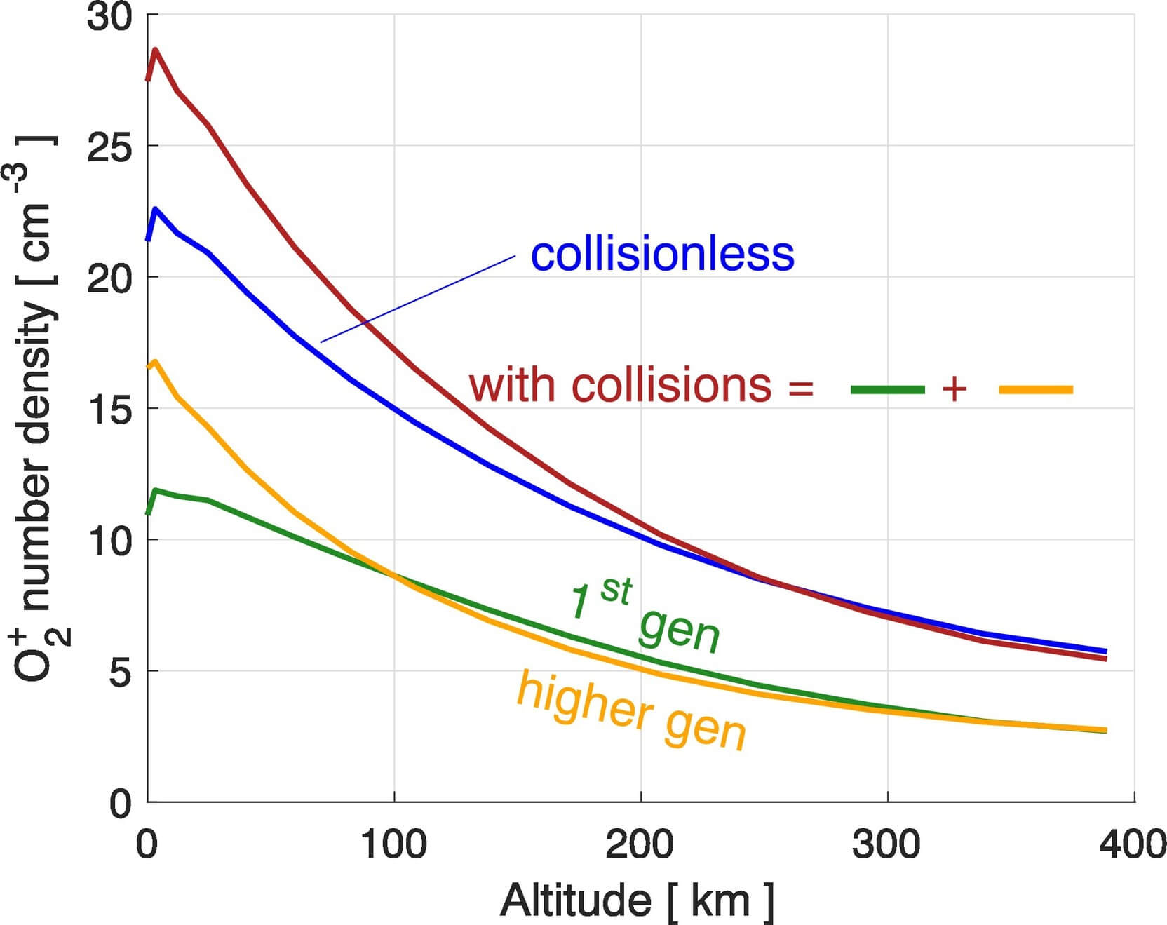
This is a test particle model built in the same group as the first hybrid model by Carnielli+ 2019. They have a follow-up paper on Constraining Ganymede's neutral and plasma properties , with the improvements of adding collisions between ion and neutral species. However, they found that this effect is only important below 200 km altitude.
In this model, ions are generated from the ionization of the neutral exosphere, whose 3D configuration is taken from the recent model of Leblanc+, 2017. The magnetic field is provided by the MHD model of Jia+, 2009.
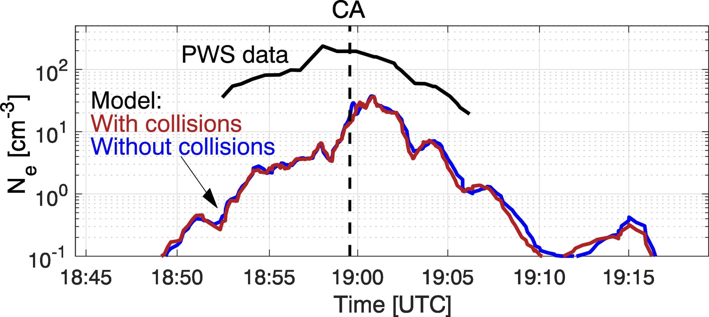
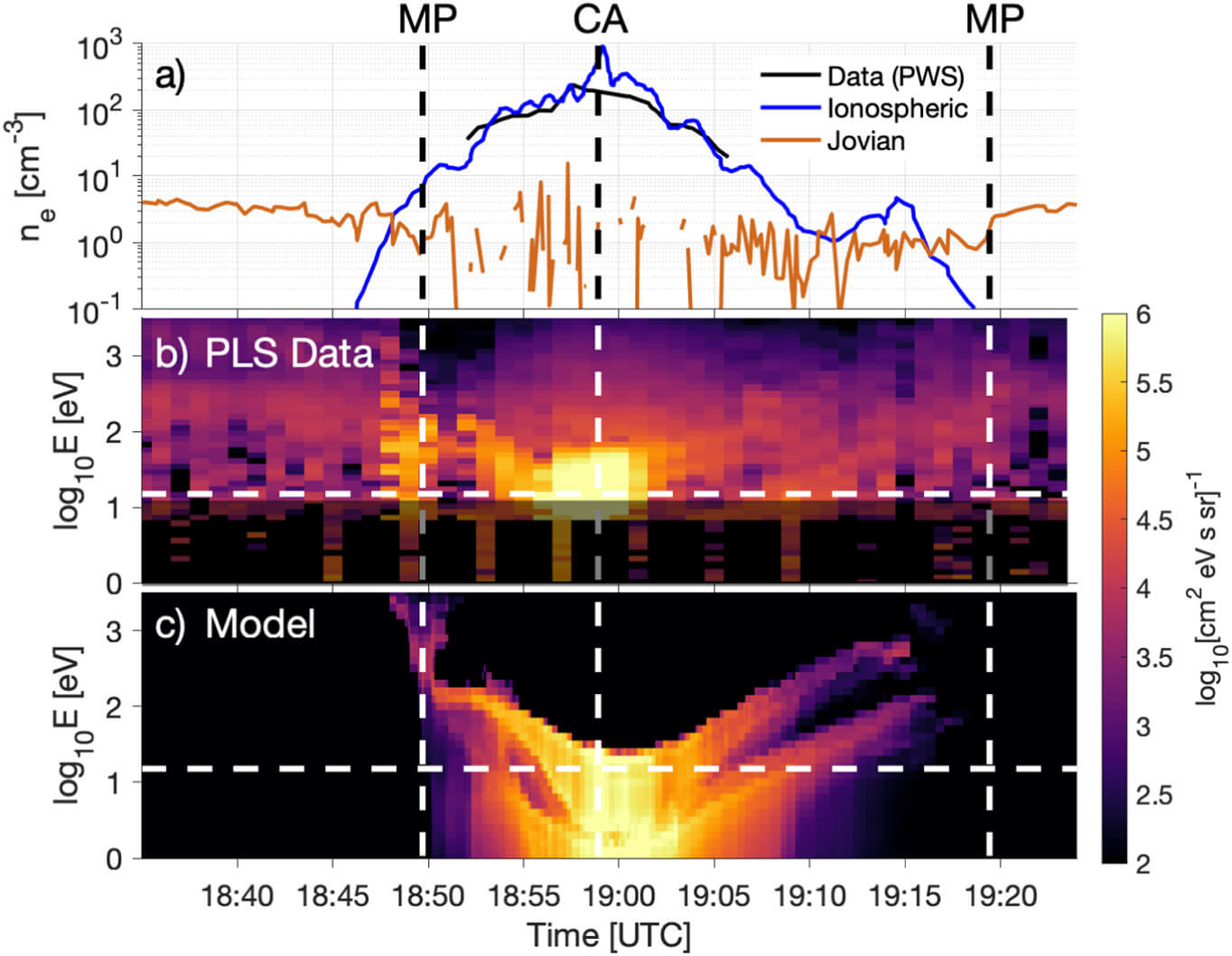
The dominant ion species found in the model is \(O_2^+\) near the surface. The ion energy distribution agrees better with observation than the electron number density, where the model gives more than one order of magnitude less than observation. They therefore suspect that the input exosphere is the likely cause for the discrepancy.
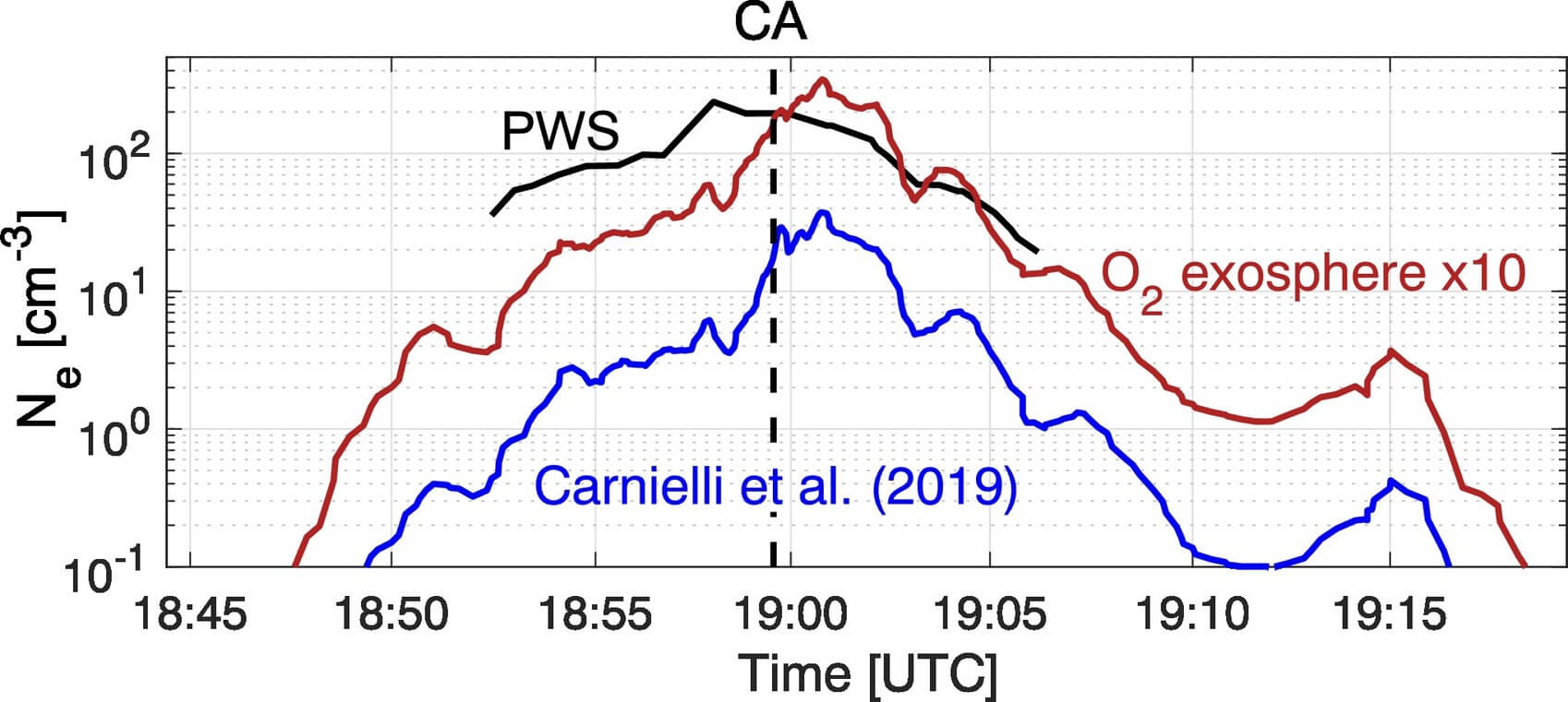
To increase the ion production rate they multiplied by 10 the \(O_2\) distribution derived by Leblanc+, 2017. This corresponds to assuming that the dynamics of molecules is exactly the same, but the ejection rate is increased by a factor of 10. This would bring the mean column density of \(O_2\), the only “observational constraint”, to \(2.44\times10^{15}\, \text{cm}^{−2}\), which is just a factor of 2 higher than the upper limit estimated by Hall+, 1998.
In the ionospheric model, the neutral exosphere is ionized by solar EUV radiation and Jovian magnetospheric electrons. On the one hand, the photo-ionization process is derived from the solar flux, which is known with a good level of confidence. On the other hand, the electron-impact ionization frequency, which is an order of magnitude larger than the photo-ionization frequency, is less certain and potentially too strong assumptions have been made in the ionospheric model. They played with it and used an asymmetric electron-impact ionization rate:
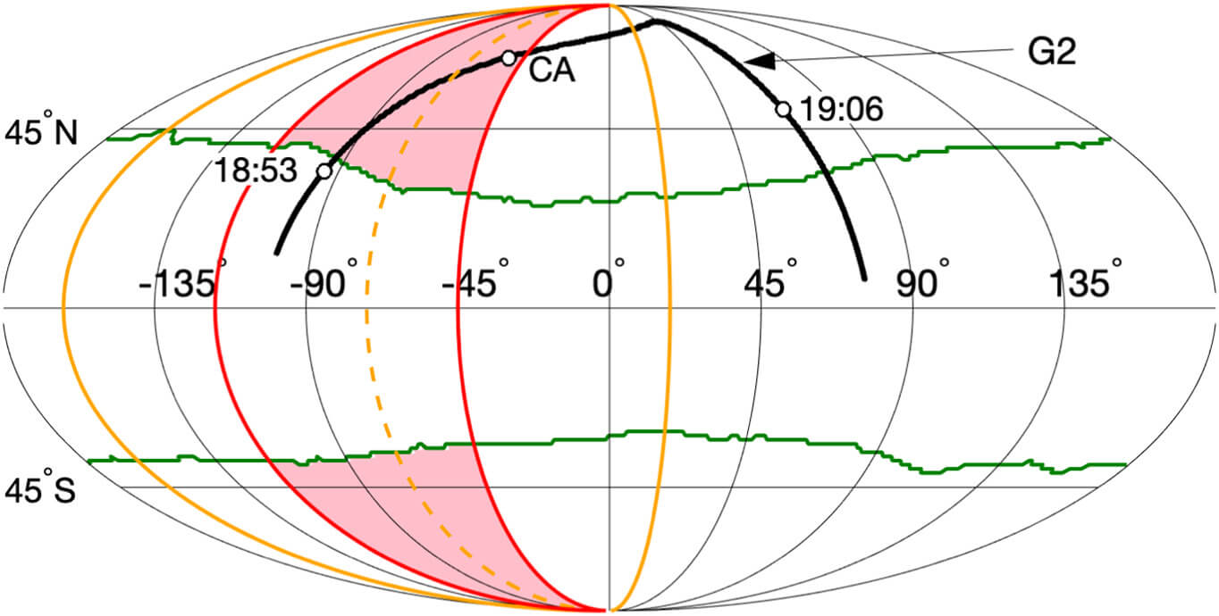
where the orange region is illuminated and the pink region has a 4 times higher ionization rate. (I don't fully understand the calculation in this part!)
This results in better comparison against the electron number density:
Electron impact calculation
MHD-EPIC, 2019-2020
| Variables | Core Boundary (\(r=0.5R_G\)) | Surface Boundary (\(r=1R_G\)) | Outer Boundary (upstream, downstream) | Outer Boundary (sides) |
|---|---|---|---|---|
| \(\rho\) | fixed, \(550 \text{amu}/cm^3\) | fixed | float | |
| \(p\) | fixed, \(0.115\textnormal{nPa}\) | fixed | float | |
| \(p_e\) | fixed, \(0.01\textnormal{nPa}\) | fixed | float | |
| \(\mathbf{V}\) | \(\mathbf{V}\perp\mathbf{B}\) | fixed | float | |
| \(\mathbf{B}\) | dipole | float[5] | fixed | float |
| [5] | For the MHD part, the float magnetic field boundary at \(r=1\) is found to be the best choice. Another option is to set the face values the same as the first layer of cells beneath the surface, which will give worse results starting from the dipole+upstream field outside the surface and pure dipole in the mantle initially. |
Test Particle Models
There are two test particle models for Ganymede in 2020: Plainaki+, 2020 on the Jovian Energetic Ion Circulation around Ganymede and Liuzzo+, 2020 on the energetic electron bombardment. The key method is the same: apply a test particle Monte Carlo model with a given EM field. The key results are similar: both models show a large-scale dichotomy in surface fluxes between the polar and the lower-latitude regions of Ganymede, with certain levels of asymmetry.