Reconnection

GEM Challenge

This 2D setup is based on Birn+ 2001, maybe with slight modifications.

The computation is carried out in a rectangular domain $-L_x/2 \le x\le L_x/2$ and $-L_z/2\le z \le L_z/2$. The system is taken to be periodic in the x direction with ideal conducting boundaries at $z=\pm L_z/2$. Thus the boundary conditions on the magnetic fields at the z boundaries are $B_z=\partial B_x/\partial z = \partial B_y/\partial z = 0$ with corresponding conditions on th eelectric fields and particle or fluid quantities. (In Vlasiator I use open boundary condition for all quantities.)

The equilibrium chosen for the reconnection challenge problem is a Harris equilibrium with a floor in the density outside of the current layer. The magnetic field is given by

where $\lambda$ is the current sheet scale size, and the density by

The electron and ion temperatures, $T_e$ and $T_i$, are taken to be uniform in the initial state. We assume the plasma $\beta = (p_i+p_e)/p_B=1$ initially.

The normalization of the space and time scales of the system is chosen to be the ion inertial length $d_i=c/\omega_{pi}$ and the ion cyclotron frequency $\Omega_i^{-1}$, where $\omega_{pi}^2 = n_0e^2/\epsilon_0 m_i$ is evaluated with the density $n_0$ and the ion gyrofrequency $\Omega_i = eB_0/m_i$ is evaluated at the peak magnetic field. The velocities are then normalized to the Alfvén speed $v_A$. In the normalized units, $B_0 = 1$ and $n_0 = 1$. Specific parameters for the simulations are $L_x = 25.6, L_z = 12.8, \lambda=0.5, n_\infty/n_0 = 0.2$, and $T_e/T_i = 0.2$. $m_i/m_e = 25$ is assumed if required.

The initial magnetic island is specified through the perturbation in the magnetic flux,

where the magnetic perturbation is given by $\mathbf{B} = \hat{y}\times\nabla\psi$, or more specifically,

In normalized units $\psi_0 = 0.1$, which produces an initial island width which is comparable to the initial width of the current layer. The rationale for such a large initial perturbation is to put the system in the nonlinear regime of magnetic reconnection from the beginning of the simulation.

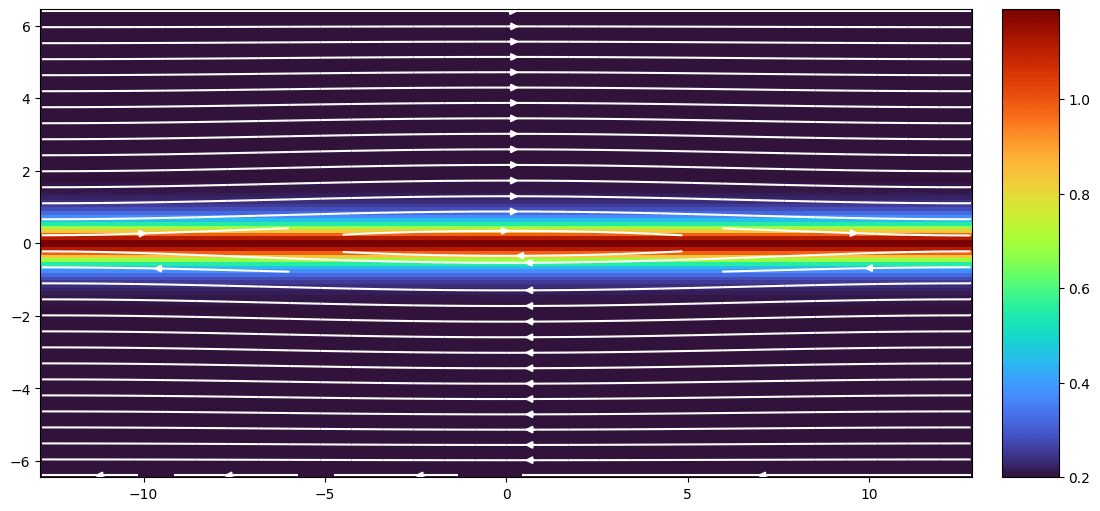
The initial setup is shown in the figure below.

Why do we need to resolve ion inertial length

Physically, electrons and ions separate at the scale of ion inertial length. Numerically, Hall term is important only when cell size is small enough to resolve the ion initial length. The reason is as follows. The Ohm's law is

Assume the typical flow velocity is Alfvén velocity: $\mathbf{U} = \mathbf{V}_A$. The Hall velocity is estimated as:

The approximation $dB\approx B$ is valid for relatively coarse grid size; for fine discrete cell sizes, this approximation does not hold, so magnetic field cannot cancel out in the following estimation. Let us now assume we can make this assumption. Then the ratio of Hall velocity and Alfvén velocity is:

Ion inertial length is also important for PIC: if particle's velocity is assumed to be Alfvén velocity, then ion inertial length is the same as ion gyroradius.

Vlasiator

Vlasiator requires SI units as inputs, so we need unit conversions. I select a reference number density scale $n_{ref} = 10\text{amu/cc}$ and magnetic field $B_{ref} = 10\text{nT}$. The dimensionless scale $\beta$ is also used to determine the unit of temperature.

The reference ion frequency in rad/s is

and then the reference ion inertial length in m, which is also used as the length scale, is

The time scale in s is the inverse of reference gyrofrequency,

Actually there is a $2\pi$ factor missing here, since we need to convert from gyrofrequency to frequency and then take the inverse for the period. However, traditionally no one did that.

The velocity scale in m/s is the Alfvén speed

The temperature scale can be derived from the magnetic pressure and $\beta$

Inserting the initially chosen values, we have a full set of conversion factors from the normalized units to SI units: $n_{ref} = 10^7\text{m}^{-3}, B_{ref} = 10^{-8}\text{T}, v_{ref} = 68960\text{m/s}, l_{ref} = 72030\text{m}, t_{ref} = 1.04\text{s}$, and $T_{ref} = 288188.74\text{K}$.

Since $\beta, T_i, T_e$ are all initially uniform, we use the boundary values to determine the temperatures. $T_i = B_0^2/n_0*β / (1.0 + T_e / T_i) = 0.83$, $T_e = 0.2T_i = 0.17$. We use the thermal speed to estimate the velocity space grid. The thermal speed scale is $V_{th} = \sqrt{k_B T_{i}*T_{ref}/m_i} = 140757\text{m/s}$. Based on experience, I set the velocity space extent to be 20 times of $V_{th}$.

Therefore, we have all the input parameters in SI units:

With $nx = 256$ and $nz = 128$, the spatial cell size is $L_x / nx=0.1 d_i$ in x and $L_z/nz =0.1 d_i$ in z. With 160 velocity space cells in each dimension, the velocity cell size is $20/160 = 1/8$ of the background thermal velocity.

Comparison

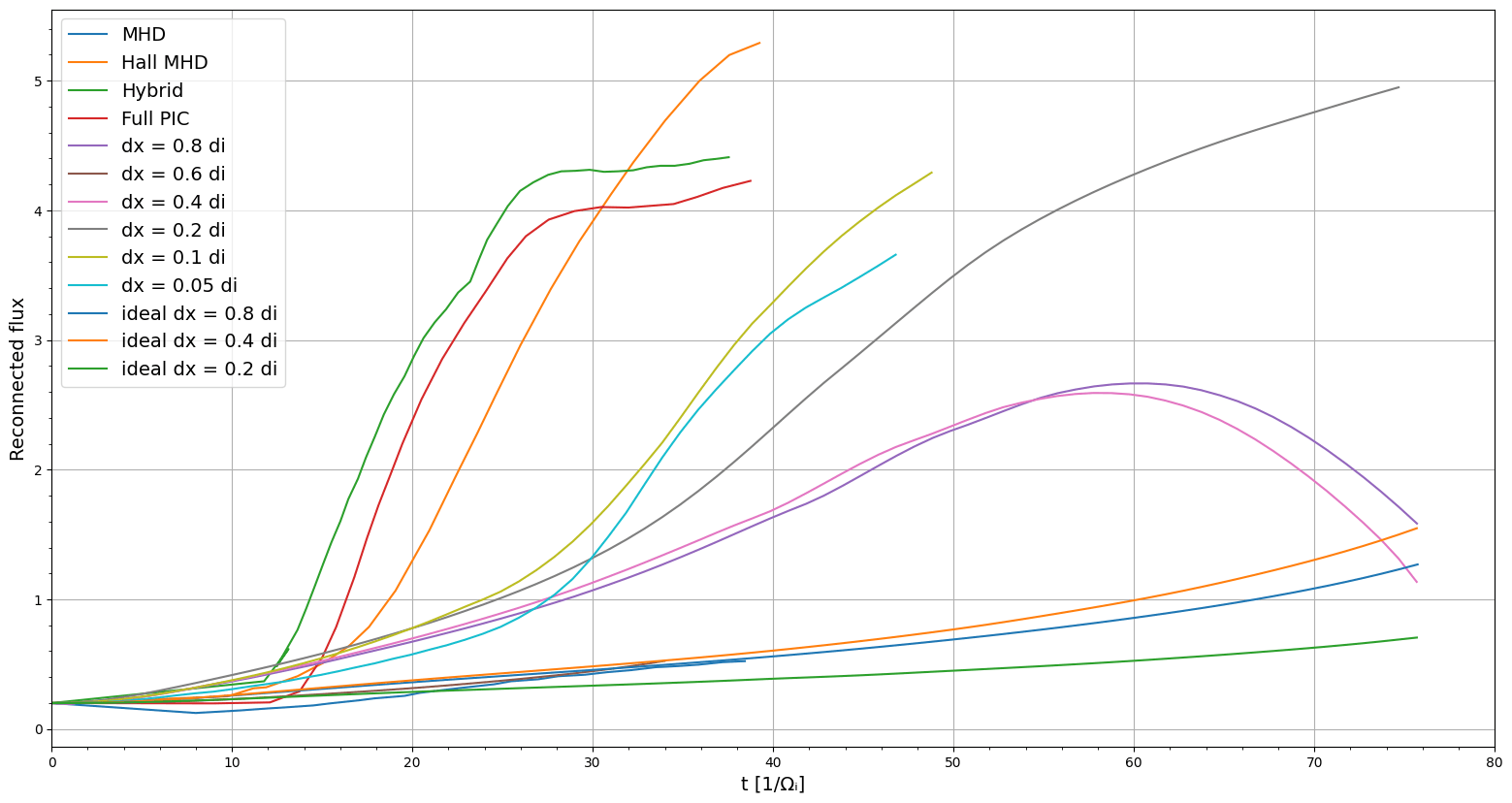
I extracted the points from Figure 1 in Birn+ 2001 and appended Vlasiator results. The normalized reconnection rates are shown below. Without the Hall term, the reconnection rate is significantly lower than others and is comparable with ideal MHD. Resolving the ion inertial length is also important to get fast reconnection rates.