Ganymede Research Log
- Lessons
- Products
- Physics
- Unit Conversion
- Coordinate System
- Numerical Schemes
- Inner BCs
- Solve Resisivity Numerically
- Outer BCs
- Local Timestepping .vs. Time-accurate
- MHD .vs. PIC
- PC Scheme
- Speed of Light
- G2
- G29
- GM/PC Coupling
- Comparison Between G8 and G28
- Magnetopause
- Reconnection, FTEs and Flux Ropes
- Potential Drop
- Neutral Exchange Rates
- ULF Wave
- KH Instability
Lessons
Collect everything into organized files and write automated scripts for future reference.
Before you test something new, make sure you can revert to the previous method. A proper version control tool is invaluable.
Be careful about unit and coordinate system conversions.
When it is a multi-variable problem, do not rush to conclusions!
Simplify tests whenever there are too many things together. Just like the design of unit tests: one thing at a time.
Products
The years of research results in many bug fixes in BATSRUS and improvements on postprocessing and visualization. The codes I write for processing and analyzing both observation and simulation results can be found at VisAnaMatlab and VisAnaJulia.
Physics
Largest moon of Jupiter (also the largest moon in the solar system), \(R_G=2634\text{km}\). Only moon to have internal magnetic field; dipole axis nearly antiparallel to spin axis.
Orbits lie very close to the rotation equator of Jupiter but tilted with respect to Jupiter's plasma sheet. Synodic period: 10.5 h. \(15R_J=15\times 71400\text{km}\); no bow shock
6 flybys of the Galileo spacecraft.
G1,G2: measured \(\mathbf{B}\) significantly increased near Ganymede, inferring an intrinsic magnetic field; sharp rotations in \(\mathbf{B}\) across the separatrices between external and connected field lines indicating strong localized currents. * Changes in energetic ion anisotropy signatures detected by Energetic Particle Detector (EPD) showed that magnetosphere significantly slows the ambient Jovian plasma in regions extending to \(\sim R_G\) away from Ganymede along the Jovian field lines connected to the moon. (Here we have inferred \(\mathbf{B}\) info.)
Detected wave modes further comfirms the existence of magnetosphere. upper hybrid resonance \(\rightarrow\) electron density \(n_e\sim 400 \text{cm}^{-3}\) above the surface (i.e. in the ionosphere), with a scale height of \(600\text{km}\approx 0.23 R_G\).
Plasma Analyzers (PLS): outflowing ions from high latitude ionosphere, indicating polar wind. This equipment is not so trustworthy.
Hubble Space Telescope: OI airglow, aurora
Alfvén wing
Refer to the original paper. Alfvén wings are a consequence of the interaction between the flow velocity and an Alfvén wave. As a magnetic field encounters an obstacle and starts to bend, Alfvén waves are launched along the field-lines away from that point. These Alfvén waves propagate along the magnetic field line with the speed \(V_A=B/\sqrt{\mu_0 \rho}\), where \(B\) is the magnetic field strength, and \(\rho\) is the plasma mass density. In addition, the plasma still advects the magnetic field with a given velocity \(V\) . The Alfvén wave, therefore, travels with an angle \(\theta=\tan^{-1}({M_A}^{-1})\), where \(M_A\) is the Alfvén Mach number, defined by \(M_A=V /V_A\) Neubauer, 1980. The flow diverts around the obstacle and forms two tubes (above and below) the object in which the flow characteristics of the plasma are altered significantly from the surrounding medium. This cavity is the low density Alfvén wing.
Ionosphere
Whether or not Ganymede has a real ionosphere is still debatable. In 2001, researchers published a paper with a conclusion that Ganymede has a bound ionosphere composed mainly of molecular oxygen ions in the polar regions and of atomic oxygen ions at low latitudes and that protons are absent everywhere. Their prediction is that Ganymede is surrounded by a corona of hot oxygen atoms.
From PWS measurements during the G1 and G2 flyby, 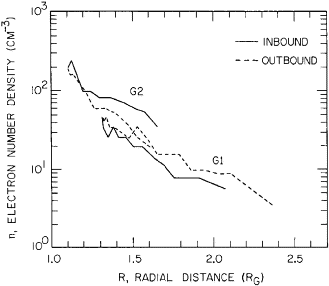
The common slope of the first mentioned triad corresponds to a scale height of 600 km and a surface density of about 400\(\text{cm}^{-3}\). This is well below the upper limit of \(4\times10^3 \text{cm}^{-3}\) obtained by [Kliore, 1998] in the radio occultation observation.
Consider two separate regions on the surface of Ganymede, the polar cap region, for which the latitude \(\lambda>45^o\) and the lower latitude regions equatorward of this limit. Neutral temperature maps published by Orton+, 1996 show a range of temperatures from about 150 K in the subsolar equatorial zone to below 90 K near the poles and in the pre-dawn sector. The \(O_2\) scale height estimated in Eviatar+, 2000 is only 21.5 km. The estimated polar cap ion density is
\[\begin{aligned} n_{O_2^+} &= 2.2 \times 10^3\,\text{cm}^{-3}, \\ n_{O_2} &= 3.5 \times 10^6\,\text{cm}^{-3}, \\ n_{O^+} &= 3.3 \times 10^2\,\text{cm}^{-3}, \\ n_{O^} &= 1.7 \times 10^6\,\text{cm}^{-3}, \\ \end{aligned}\]In the closed field line region, the magnetospheric thermal plasma density can be expected to be very low in this region, because of the inaccessibility of closed drift paths to injected Jovian particles and the paucity of local plasma sources. In the low-latitude regions of Ganymede, the dayside temperature can be as high as 140–150 K.[1]
| [1] | High-low is always relative. Keep in mind that this \(10^2\) K temperature is in fact very very low compared to the background energetic ions that contribute most of the pressure! |
photo-ionization
dissociative recombination
electron impact
MHD
Magnetohydrodynamics (MHD) equations are presently the only system available to self-consistently describe large-scale dynamics of space plasmas, and numerical MHD simulations has enabled us to capture the basic structures of the solar wind plasma flow and transient phenomena. The modern MHD codes can successfully solve both in time accurate and steady state problems involving all kinds of discontinuities. Different from the usual computational fluid mechanics, the MHD scheme has to be designed so as to guarantee the divergence free constraint of the magnetic field in two or three-dimensional MHD calculations. It is well-known that simply transferring conservation law methods for the Euler to the MHD equations can not be supposed to work at default in maintaining the divergence-free of magnetic field. The \(\nabla\cdot\mathbf{B}\) error accumulated during the calculation may grow in an uncontrolled fashion, which can result in unphysical forces and numerical instability [Tóth, 2000; Jiang+, 2012a][2]
| [2] | R.L Jiang at Nanjing University has an AMR MHD code which should be similar to BATSRUS. |
Resistivity
Resistivity calculation: I calculate the peak resistivity based on the estimation that within range \(r\in[r_G,1.05r_G]\), the total conductance is \(2S\), which means the resistance is \(0.5\Omega\).
\[ R=\eta \frac{l}{A}=\int_{1R_G}^{1.05R_G}\eta \frac{dr}{4\pi r^2} \]Assume that the resistivity changes linearly, \(\eta=Ar+B\),
\[\begin{aligned} &A\cdot 1R_G + B = \eta_H, \\ &A\cdot 1.05R_G + B = 0 \\ \Rightarrow &A=-20\eta_H/R_G,\ B=21\eta_H \end{aligned}\]So in normalized radius \(r^\prime\),
\[ \eta=-20\eta_H r^\prime +21\eta_H. \] \[\begin{aligned} R&=\frac{1}{4\pi}\int \frac{\eta(r)}{r^2}dr =\frac{1}{4\pi}\int \frac{Ar+B}{r^2}dr=\frac{1}{4\pi}\Big[ A\int\frac{dr}{r}+B\int \frac{dr}{r^2} \Big] \\ &=\frac{1}{4\pi}\Big[ A\ln{r}-B\frac{1}{r}\Big]\big|_{1}^{1.05}=0.5\Omega \end{aligned}\] \[\begin{aligned} \frac{1}{4\pi}\Big[ -20\frac{\eta_H}{R_G}\ln{21/20}-21\frac{\eta_H}{R_G}(\frac{1}{1.05}-1)\Big]=0.5 \\ \Rightarrow \eta_H=2\pi*R_G/(-20\ln{1.05}-21/1.05+21)=6.3334\times10^8 \Omega\cdot\text{m} \end{aligned}\]However, in BATSRUS, the units of resistivity is \(\eta/\mu_0\),
\[ \eta_H = \frac{6.334\times10^8}{4\pi\times10^{-7}}=5.04\times10^{14} \]Inside the body,
\[\begin{aligned} \mathbf{j} = \sigma (\mathbf{E}+\cancel{\mathbf{u}\times\mathbf{B}}) \\ \frac{\partial\mathbf{B}}{\partial t}=-\nabla\times\mathbf{E}=-\nabla\times(\eta\mathbf{j})=-\nabla\times(\frac{\eta}{\mu_0}\nabla\times\mathbf{B}) \end{aligned}\]If \(\eta=const.\), then
\[ \mu_0 \sigma\frac{\partial\mathbf{B}}{\partial t}=\nabla^2\mathbf{B} \]This is same as shown by Eq.(1) of Zimmer's Europa paper.
I have non-uniform resistivity inside the body, so things get complicated.
I don't know if dipole field satisfies \(\nabla^2\mathbf{B}=0\).
Outside the body,
\[ \frac{\partial\mathbf{B}}{\partial t}=-\nabla\times(\eta\mathbf{j} - \mathbf{u}\times\mathbf{B})=\nabla\times(\mathbf{u}\times\mathbf{B})-\nabla\times(\eta\mathbf{j}) \]The right-hand side is treated in ModFaceFlux.
The induction effect of a conducting core. The physical model is that you have a very high conductivity core region and a low conductivity mantle region. Because of the high conductivity of the core, we can treat it as a perfect conducing core with a dipole field generated from a dynamo. If you set \(\eta=0\) in the mantle region (low resistivity), the B field is then fixed in the mantle so that it acts like a perfect conducting sphere with radius \(r=1R_G\). Xianzhe mentioned in his Mercury paper a comparison between a conducting core and a purely resistive body (without a conducting core). My understanding is as follows: if you reach a steady state with a given resistivity profile, you get a curl-free steady B (at least for the mantle region).If then you use another resistivity profile to get a new steady state, it is still unclear what resistivity do in the process. What Xianzhe did in the Mercury simulation is that (at least I believe) he continued the steady state solution that is reached by including a conducting core in two ways: one still with a conducting core (by keeping the resistivity profile as shown in the plot) and a pressure enhancement, and the other without a conducting core (by setting very high resistivity near the surface of the core?) In this way you cannot get strong current near the core surface so no induction effect. You see what I mean? The absolute resistivity value may be unimportant in a steady state solution.
Yuxi said he once asked Xianzhe about why we are not considering induction effect for Earth and Jupiter, for example. Xianzhe responded that the reason is the core of Earth is relatively small comparing to its size of magnetosphere.
Based on my understanding here, I need to modify my resistivity profile at the core boundary. I should extend zero value to about \(0.52R_G\).
Fit to the dipole moments and induced magnetic field
The induced dipole field is produced as a result of interaction between the time-varying Jovian magnetic field and the high conducting core. See the Europa paper. In our simulations, the upstream conditions are set to fixed, so this effect is missing. As a compensation, we analytically calculate the induced dipole field and add to the intrinsic dipole field.
| Flyby | \(M_z\) [nT] | \(M_y\) [nT] | \(M_x\) [nT] | \(B_x^{bk}\) [nT] | \(B_y^{bk}\) [nT] | \(B_z^{bk}\) [nT] | \(v\) [km/s] | \(\rho\) \([\mathbf{amu}/\mathbf{cm}^3]\) | \(P\) [nPa] |
|---|---|---|---|---|---|---|---|---|---|
| G1 | -716.8 | 82.5 | -24.7 | 6 | -79 | -79 | 140 | 28 | 1.9 |
| G2 | -716.8 | 80.0 | -29.3 | 17 | -73 | -85 | 140 | 28 | 1.9 |
| G7 | -716.8 | 14.0 | -20.9 | -3 | 84 | -76 | 130 | 28 | 1.9 |
| G8 | -716.8 | 51.8 | -18.0 | -11 | 11 | -77 | 140 | 56 | 3.8 |
| G28 | -716.8 | 17.0 | -19.3 | -7 | 78 | -76 | 140 | 28 | 1.9 |
| G29 | -716.8 | 84.2 | -18.4 | -9 | -83 | -79 | 140 | 28 | 1.9 |
From [Kivelson+ 2002] Table V, the dipole moments are fitted from G1, G2, and G28. For all the flybys, magnetic fields are fitted as follows:
\[\begin{aligned} \alpha = 0.84 \\ M_{x,0}=-h_{1}^1 = -22.2 \text{nT},\quad M_{y,0}=g_{1}^1 = 49.3 \text{ nT},\quad M_{z,0}=g_{1}^0 = -716.8 \text{nT} \\ G1: M_x = M_{x,0} - \alpha*0.5*B_x^{bk} = -24.72 \text{nT},\ M_y = M_{y,0} - \alpha*0.5*B_y^{bk} = 82.47 \text{nT} \\ G2: M_x = M_{x,0} - \alpha*0.5*B_x^{bk} = -29.34 \text{nT},\ M_y = M_{y,0} - \alpha*0.5*B_y^{bk} = 79.96 \text{nT} \\ G7: M_x = M_{x,0} - \alpha*0.5*B_x^{bk} = -20.94 \text{nT},\ M_y = M_{y,0} - \alpha*0.5*B_y^{bk} = 14.02 \text{nT} \\ G8: M_x = M_{x,0} - \alpha*0.5*B_x^{bk} = -17.58 \text{nT},\ M_y = M_{y,0} - \alpha*0.5*B_y^{bk} = 44.68 \text{nT} \\ G28: M_x = M_{x,0} - \alpha*0.5*B_x^{bk} = -19.26 \text{nT},\ M_y = M_{y,0} - \alpha*0.5*B_y^{bk} = 16.54 \text{nT} \\ G29: M_x = M_{x,0} - \alpha*0.5*B_x^{bk} = -18.42 \text{nT},\ M_y = M_{y,0} - \alpha*0.5*B_y^{bk} = 84.16 \text{nT} \end{aligned}\]What I found from this calculation is that \(M_y\) for G8 is off by \(7\,nT\).
At some point I questioned the dipole fit. I had an idea of checking the dipole with G2. The box output with ipict=1 is the sum of the dipole and background field. Subtract the background field, and you can feel how strong is the dipole. I expect this to be very close to Galileo data. Use this to verify my dipole moments. I also did a dipole test and collected the results in a PDF.
There is a point when I get better results with the correct dipole calculation and a different resistivity number.
Electron pressure equation
After I had partly success with the ideal MHD tests, I moved on to include an independent electron pressure equation into the model. Previously we used a fixed \(P_e/P_i\) ratio 1/5.
MHD with Pe and hyperbolic cleaning seems to work fine (even better for steady-state B comparison!). The ion/electron pressure ratio is larger than 5 inside the magnetosphere
Reconnection rate
How to calculate the reconnection rate? \(\exp{\gamma t}\)
Generation of magnetic field
Gabor mentioned to me one thing: electron pressure gradient is a potential possible way of generating magnetic field without the existence of magnetic field. Actually this is discussed a lot in astrophysics and is regarded as one key mechanism of creating magnetic field.
Magnetic field topology classification
There are two built-in ray tracing schemes in BATSRUS; there is also a field line identification algorithm described in Alex Glocer's paper. Paul Cassak had a student working on this as his PhD thesis.
Using the status variable from BATSRUS's field tracing, we can identify open/closed field lines.
I once spent several days to debug the field line tracing scheme for my Ganymede runs; it turned out that an incorrect setup of the minimum radius led to an infinite loop. On a second thought, the original design of related modules in Fortran is the root cause why these bugs are hard to find.
I once thought about the idea of helicity, but soon gave it up:
magnetic reconnection can be regarded as a process of conversion between different forms of magnetic helicity, while the total magnetic helicity is conserved in the process (Woltjer 1958; Taylor 1974; Wright \& Berger 1989).
Helicity is a "quasi-conserved" quantity in Hall-Resistive MHD.
\(\mathbf{E}^\prime = \mathbf{E} + \mathbf{v}_e\times\mathbf{B}\)
\(\mathbf{E}^\prime = \mathbf{E} + \mathbf{u}_i\times\mathbf{B}\)
\(\mathbf{E}^\prime\cdot\mathbf{J}\)
\(J/B\)
\(\nabla\cdot\mathbf{v}_e\)?
\(T\)
None of the above works well in the simulations.
Gravity
For solving the density diffusion problem at the inner boundary, Gabor suggested turning on gravity. This has little effect on the results.
Why is it challenging?
Nearly all the approximations and tricks I use in my Ganymede simulation is to deal with the multi-scale problem.
Unit Conversion
Most studies use SI units. Some old studies use CGS units.
Coordinate System
Commonly we are using GPhiO coordinate system.
Numerical Schemes
BATSRUS has the option of using conservative scheme or nonconservative scheme. The difference lies in whether we are solving the pressure equation or the energy equation. According to Gabor's experience, these two behave differently especially for shocks. I have seen that in Ganymede's case, solving the pressure equation will lead to an increase of density along the Alfvén wing edges, which does not appear when solving the energy equation. Physically, the shock discontinuity is described by the conservation laws. Using a pressure equation indicates that we assume some kind of physical processes, e.g. adiabatic, which may not hold across the discontinuity. The default choice for BATSRUS is to only apply nonconservative scheme near the Earth, which makes sense in this regard.
In Jia+, 2008, they solved the pressure equation everywhere; in Duling+, 2014, they solved the energy equation everywhere; in Fatemi+, 2018, the hybrid model seems to use pressure equation or equivalence; in Zhou+, 2019 and Zhou+, 2020, I solved the energy equation everywhere.
Fully explicit method
If we update everything explicitly, the large density inside the body to reduce large Alfvén speed for timestep calculation.
Semi-implicit method
However, with semi-implicit method and solid body this is no longer true.
Happened to find that my timestep for the cell inner BC Hall MHD run is incredibly small for the pole region inside \(r=1\), the time step is about \(\sim10^{-6}s\)! Yuxi told me this is because of the resistivity. Remember you need to switch to semi-implicit scheme for time-accurate mode? This is the reason! Also, the smallest timestep shows up in one layer of cells below \(r=1\) when I had coarse axis turned on. Just think about this: things get slowed down at \(r=1\)!
Solution: use semi-implicit scheme in both local timestepping and time-accurate mode.
Maybe the implicit timestep inside 0.01s is too large? Remember this would effect accuracy, but not stability.
Div B cleaning
8 wave scheme
Hyperbolic cleaning
why there's nonzero flux in the mantle cell at the very first timestep. I found it. Flux_V is nonzero because of #HYPERBOLICDIVB. This is the reason for local extreme inside the mantle. I should read about the original paper about hyperbolic cleaning and Gabor's paper on solving divB problem.
In DivB constaint techniques, there is another simple idea in the literature. Instead of solving the magnetic induction equation alone (3 equations with 3 unknowns), we can solve two of them and add the \(\nabla\cdot\mathbf{B}=0\) to it. Or in a similar way, we can find the least square fit to the 3 unknowns with 4 equations.
Currently there is an inconsistency of \(\nabla\cdot\mathbf{B}\) in the initial condition. No matter how hard you try with hyperbolic cleaning and eight-wave scheme, you cannot get rid of the divergence at the inner boundary! Imagine if you are running with a CT scheme, even though no numerical divergence is being created, you will still suffer from the unphysical initial condition.
Hall MHD
Yuxi said the reason my face Hall MHD gives wrong solution may be instability. I can try to increase the HallCmaxFactor and decrease the timestep inside \(r=1\).
HallCmaxFactor also has an effect on the results. If I use \(0\), then the results becomes unstable gradually.
I will try to test on the optimal value for these two. I will test on G2 and G8, first the timestep, then the HallCmaxFactor.
Inner BCs
Cell .vs. face
At \(r=1R_G\), we have the option of using user-defined cell BC and solid body face BC. The cell BC is developed for mercury as part of the work of including a resistive body. This approach is like a hack into the numerical solver: it overwrites the cell center values below the surface, which is not compatible with the hyperbolic cleaning and the semi-implicit scheme (for some unknown reasons). This is dangerous and error-prone.
On the other hand, Bart introduced #SOLIDBODY command for the solar applications. I took advantage of that and create a face BC at \(r=1R_G\): during the explicit update phase, a face boundary is placed at \(r=1\) so the MHD equations are solved only in region \(r>1\); during the implicit update phase, the face boundary is turned off and the inner boundary is now at the core, and we only solve for \(\eta\mathbf{j}\) term in the magnetic induction equation.
The cell BC can be second order while the face BC is only first order. During the initial phase of transitioning from cell to face inner BC, I felt that the face BC is not robust enough. As I become more and more familiar with the method, the advantages of face BC surely makes it a better option than cell BC.
MHD boundary conditions
We need to set the boundary conditions for \(\rho,\mathbf{U},\mathbf{B}\) and \(P,Pe\). Currently in BATSRUS, cell boundary can only be applied at real mesh boundaries, and we can only use face boundary inside the mesh domain. Due to the lack of theoretical support, I have to do a lot of tests and numerical experiments.
For the density, we use fixed BC with \(\rho=550\) amu/cc. The idea is that we want to mimic a cold dense plasma source. If the density is set too high, all the densities inside the magnetosphere are high, and there's no density drop across the magnetopause.
I once tried a steady state test with surface density down to 100 amu/cc. The magnetic field significantly changed. I can see a plasma cavity at dayside, but the magnetic field comparison becomes worse probably because the inner pressure I set was too large, such that the magnetopause got expanded.
Actually one idea to test the density only is to completely remove the magnetic field and focus on the hydrodynamics part.
For the high resolution runs (AMR3), the density peak at dayside near the surface becomes more of an issue. Also, in Hall MHD, even if the Hall region is set to \(r=1.05\), the peak at the tail near the surface becomes another issue. In any case, the flow pattern is consistent with the prescribed boundary condition, but not necessarily be correct in nature.
Duling+, 2014 and Toth+, 2016 uses float density.
For the velocity, we have three choices:
absorb, which means that plasma velocity can only goes into the body;
reflect, or solid, which means that plasma flow cannot penetrate the surface;
\(\mathbf{B}\) dependent, which means that we remove the plasma velocity parallel to the surface, but keep the perpendicular components.
For the magnetic field, we use float at the surface.
For the pressures, we use either float or fixed. I am not sure if fixing both density and pressure will create an overspecified system.
If I use float P at r=1, the pressure at the tail near the surface would reach as high as 25 nPa. If I use fixed, then it only reach about 12 nPa. While keeping everything else the same, using fixed pressure has much better magnetic field comparison.
On a coarse grid (0.3 million cells), a bunch of tests are performed. While the third velocity BC can give nice magnetic field comparisons with a proper resistivity, it does not give a physically meaningful plasma flow pattern: there is always a source point on the upstream front, and the flow moves towards the tail at relatively high speed around the flanks. The reflect U BC can give nice flow pattern, but the magnetic field comparison is off due to the fact that the magnetosphere gets expanded.
At a certain time for the solid BC runs, I get inflow at the dayside inner boundary, and a small pressure bump near the surface.
The absorb BC, which is also used by Duling+, 2014 and Tóth+, 2016, also gives wrong flow pattern on the flanks.
The flow pattern issue is also present in some Cartesian grid ideal MHD runs, indicating that it has nothing to do with the grid geometry.
Tests of different resistivity profiles (\(\eta_{max}=5\times 10^{11}m^2/s\), \(\eta_{max}=8\times 10^{11}m^2/s\), \(\eta_{max}=3\times 10^{11}m^2/s\)) shows that the whole flow pattern is not sensitive to \(\eta\mathbf{J}\). All runs show similar flow pattern in the equatorial plane: there's a spurious return flow on the two sides at \(r=1\).
I have repeatly confirmed that one quasi-steady solution with the given BC can convert to others by changing the inner BC setup.
Besides, I have also tried to implement the insulating BC described in Duling+, 2014. On a coarse grid, this BC gives pretty good magnetic field comparison. However, I gave it up later because I did not know how to make it work in parallel with the FFT computation.
I always believe there are still inconsistencies in the boundary setup. None of the existing models provide a correct description of the inner boundary, and in fact how can believe that an MHD model can have an inner boundary that is actually the solid moon it self?
I have an idea of half absorb half reflect U.
Core boundary condition
At the core boundary, we only need to set magnetic field \(\mathbf{B}_1\). I used fixedb1/fixedb1_semi before. I should use zerob1.
Solve Resisivity Numerically
For semi-implicit scheme, the larger \(\eta\) I use, I longer it will take for a certain number of timesteps. This means that larger resistivity gives stiffer problem to solve.
One problem I encounter with 40000 steps in steady state run with \(\eta=3\times 10^{11}m^2/s\). From \(P_{max}\) .vs. timestep plot, I can see clear periodic oscillations indicating it is not converging. The streamline plot in \(y=0\) plane shows unphysical behavior near the pole region: it is too large, up to about 130km/s. The compare with Galileo still has an off-set for the magnetopause position. \(\eta=3\times 10^{11}m^2/s\) test: no spurious flow pattern in the equatorial plane at the sides; the Galileo comparison is ok. I realize one thing: the resistivity profile I use in Bad results. Even \(\eta=1\times 10^{11}\text{m}^2/s\) results in a small magnetosphere than Galileo observed. The even smaller \(\eta\) run is worse. However, if I turn on Hall MHD, the magnetosphere will expand. G8, \(\eta=0\) run. Physically, this is equivalent to a perfect conducting sphere with \(r=0.5R_G\)? No, not that easy. I get very small magnetosphere, the standoff distance is about 1.8, and the tail reconnection region center distance is about 2.5. This is consistent with my previous tests that the smaller the resistivity is, the smaller the magnetosphere is. However, when I check the \(b_1\) components in \(0.5 For the G8 run with cell inner boundary, I found that \(\eta=5\times 10^{11}m^2/s\) seemd to be a proper number. Checked my coarse grid runs with \(\eta=5\times10^{11}m^2/s\) for cell and face based solution for 750 steps. In general, they looked similar. There are differences, but I can't tell which one is correct simply from these variable comparisons. solid timestep \(0.5\times10^{-3}s\), \(\eta=3,2,1\times10^{11}m^2/s\). Pick the best fit, run for longer! Still testing on the proper \(\eta\) value. \(1\times10^{11}m^2/s\) is not good; \(3\times10^{11}m^2/s\) gives slightly larger magnetopause. The face innerBC comparison of Hall MHD for G2 and G28 \(\eta=3\times10^{11}m^2/s\) are almost perfect. However, when I turned to PIC, the whole magnetosphere expands so I get much worse results... Checked the cell innerBC results with \(\eta=3,4,5\times10^{11}m^2/s\), and found that \(\eta=3\times10^{11}m^2/s\) is the best fit. Two Say we are solving \(\frac{\partial \mathbf{B}}{\partial t}=\eta\nabla^2\mathbf{B}\). The timestep limit requires that However, this is only true for the smallest cells inside the body! Resistivity at the boundary cells is crucial in getting the correct solution! We need to have at least 2 layers of 0 resistivity cells to produce the correct \(\mathbf{B}_1\) field around the core boundary. If the resistivity in the nearest physical cell is not 0, then even if the resistivity in the ghost cells are zero, the boundary face would have non-zero resistivity and corresponding non-zero electric field. This will give totally wrong behavior for the magnetic field topology. read two papers: one on Europa for the idea of induced magnetic field, another on Mercury for the property of resistivity. I found that the solidtimestep inside \(r=1\) is the reason for the wrong results: I picked a too large timestep \(10^{-2}\)s. Maybe some value around \(10^{-4}\)s is better. Source terms can be used to include physical processes that MHD would otherwise not model or to model sources or sinks of MHD quantities. Mass loading is the physical process in which newly created charged particles become part of an ambient plasma flow via electromagnetic forces. The processes of photoionization and electron impact ionization add new mass to the plasma, while charge exchange reactions may or may not add mass. Ionization creates an electronion pair — a source of new charge and mass for the plasma. Recombination acts as a sink of plasma in a similar way. Charge exchange on the other hand, exchanges a thermalized plasma ion with a neutral particle. In the process, mass may be added (asymmetric charge) or it may not (symmetric charge exchange). An example of charge exchange which adds mass is the accidentally resonant charge exchange reaction between hydrogen and oxygen. The forward reaction of the \( H^+ + O \rightleftharpoons H + O^+ \) charge exchange process is a typical example of mass addition without creating new charge. An example of the special case of no new mass being added is the resonant charge exchange between atoms and their corresponding ions (such as \( O^+ + O \rightleftharpoons O + O^+ \). In this case, there is neither new charge nor new mass added to the plasma, however the momentum and energy can change. The reaction results in a "friction" like force on the plasma as the ion moving with the plasma is replaced by a neutral at a different velocity. One can obtain the formulation of the source terms for MHD by starting with the Boltzmann equation [e.g., Gombosi et al., 1996]. Terms are formulated for this equation and then appropriate velocity moments are taken, resulting in the mass loading and friction source terms. The source vector (in the conservative form of equation 2.18) can be written as [Gombosi et al., 1996: Combi et al.. 1998]: where \(\dot{\rho}\) is the net mass addition rate (production minus loss due to ionization and charge exchange), \(\eta\) is the coefficient of frictional interaction between the plasma and the neutral gas due to charge exchange reactions and \(L_e\) is the coefficient associated with electron recombination. Note that in the first bracket the first term in each line is associated with mass addition (ionization and charge exchange) and the second is due to friction (charge exchange). The second bracket represents the loss terms associated with recombination. It is interesting to examine the first term (associated with mass addition due to ionization and charge exchange) in both the conservative and the primitive forms. Table below shows the terms in the momentum, pressure and energy equations for mass loading where the velocity of the ionized neutrals is zero. From the conservative form it is clear what change the total momentum and energy of the plasma undergo. With the neutral at rest the neutral has no momentum and no energy that it can add to the plasma when it is ionized. The primitive form of the momentum equation shows that while the plasma momentum is conserved, the mass addition must be offset by a decrease in the plasma velocity. This process heats the plasma as seen by the source term in the pressure equation. Ionization source terms in primitive and conservative form: Mass loading/loss: photo-ionization dissociative recombination electron impact I have found the recombination process in What I have in mind is similar to what's been described in Duling+, 2014. From a modeling perspective, we need to specify the \(O_2\) number density distribution, calculate the production rate, loss rate and collision frequency according to the formulas, and then add to the mass and momentum equations. As a starting point, I can use a hydrostatic assumption for the neutral atmosphere, with uniformly distributed \(O_2\). If I believe that a denser atmosphere is true from Carnielli+, 2020 and use a column density \(N_n = 2.44\times10^{15}\, \text{cm}^{−2}\) and scale height \(H = 250\) km, then From Yash's Jupiter paper, where \(C_i\) is the ionization rate (specified to \(10^{−4} \text{s}^{−1}\) in the simulations) and 16 amu is taken to be the average mass of the heavy ions present in Jupiter's magnetosphere. The source terms for the mass continuity, momentum, total energy and thermal energy equations (Hansen, 2001): where \(C_\text{ex}\) is the charge-exchange rate, \(\mathbf{U}_n\) is the Keplerian velocity of neutral particles orbiting Jupiter, and \(\alpha_\text{rec}\) is the recombination rate, which is set to 0.[3] [4] [5] In a steady state, when we equalize the production with loss, the plasma number density at the surface should be or, assuming all \(O_2^+\), the mass density will be \(1.7\times 10^5\,\text{amu}/\text{cc}\). This is very large compared to the previous fixed density \(550\) [amu/cc] in our runs, or the \(\sim 10^3\) [amu/cc] in both Duling+, 2014[6] and Fatemi+, 2018.#SOLIDSTATE at first is that the region \(rPARAM.in starts from \(r=0.95\). This may have an influence on the results. I tried \(r=0.98\) for another test. Also, Duling+, 2014 uses \(\eta=1.6\times 10^{10}\text{m}^2/s\) at the surface. I also want to test that.PARAM.in files only differ in solid timestep: one used \(5^{-4}s\) and the other used \(1e^{-4}s\). The larger timestep run gives better comparison with Galileo data.
Better Inner BC
Equation Primitive Form Conservative Form Momentum \(-\dot{\rho}\mathbf{U}\) 0 Pressure \(-\frac{1}{2}\dot{\rho}\mathbf{U}\) - Energy - 0
UserSaturn, impact ionization, charge exchange and recombination in UserMars. For Mars, there are currently a 4 species module and a 5 fluids + Pe module. The latter is inherited from the former one.
[3] The mass and momentum equations are consistent with K.C.Hansen's thesis. The energy equation in Yash's paper is wrong, but the pressure equation is probably correct.
[4] Initially I made many mistakes on the velocity. I don't quite understand the terms especially in the pressure equation: why does it look like a source term?
[5] \(C_\text{ex}\) is the same as \(\eta\) in K.C's thesis; \(\alpha_\text{rec}\) is the same as \(L_e\).
As an estimation, the source term in the mass equation gives [6] See the discussion and some of my opinion here.
For the coarse grid run with about 0.3 million cells, the time step at the surface is on the order of \(10^{-2}\)s. For 1000 steps in local timestepping, the increase in density is about 700. This is very small compared to the expected value above. I have no idea how long it takes to reach equilibrium or will it ever reach equilibrium.
After normalization, the unit for density is [amu/cc] and for velocity is [R/s].
For my specific problem, I need to have a feeling about the surface density, pressure and temperature in equilibrium. If I trust Fatemi+, 2018's result, than it means that the thermal pressure does not matter much. Similar things may happen in Duling+, 2014. According to my simple test, the upstream pressure has little influence on the magnetic field topology.
Now that this is partly working, the next thing I would like to add is the term in the electron pressure equation. This may not matter much, but it would be better if I have those electron source/sink terms included.
Single fluid description is clearly a deficiency here, but the question is: is it enough or do we need more complex physical description? In terms of overall magnetic field topology, this probably won't matter much; but is it crucial for energetic species near the moon? Use MHD just to simulate the thermal plasma background, and use PIC to get the energetic part done?
Outer BCs
There are two types of outer boundary conditions: cell BC (#OUTERBOUNDARY) and face BC (#BOXBOUNDARY).
Local Timestepping .vs. Time-accurate
I found that the local timestepping mode gives smaller magnetosphere than the time-accurate mode. There's no true steady state, especially after the inclusion of Hall MHD, and the detailed shape of the magnetopause is changing constantly.
MHD .vs. PIC
In general, PIC gives smoother results than MHD in MHD quantities, with/without extra artificial smoothing in PIC. The reason we have E field smoothing is to reduce the noise in the particle solutions.
PC Scheme
After a bunch of tests, we found that the original implicit PIC scheme is noisy especially in electric field, and it would create numerical waves inside the magnetosphere. We suspected that it owed to the fact that neither the momentum nor the energy is conserved. This is why we switched to the new energy and charge conserving scheme in the next step.
Speed of Light
In G8 PIC simulation, electron thermal velocity (\(uxs0,uys0,uzs0\)) in certain regions is larger than the speed of light (1000km/s) I set in the iPIC simulation. The code can still run, but this is usually a sign of error. Throughout the 600s, the velocity profile is, to me, very steady. There are some noise in the upstream region (left), but I think it's fine.
When I increase the speed of light from 1000km/s to 2000km/s, I can see more FTEs!
G2
G2 velocity plot shows much larger velocity components than the hydrogen ion observation. It is strange that the heavy ion observation inside the magnetosphere is missing. There is estimation in William's paper for the maximum ion velocity inside the magnetosphere for G2, which is about \(25 \sim 45\) km/s.
G29
For the G29 flyby, I get a shift in B for the trajectory comparison, same as Xianzhe's previous model, but different from [Duling+ 2014] and the hybrid model from Berkeley.
G29 time shift, try adding a negative Vy (e.g. -30km/s) to see if there's any shift.
GM/PC Coupling
I went through the commands of GM-PC coupling with Yuxi. Now it seems to work. I need to go over the commands again and ask Yuxi to complete the PARAM.XML. Take notes!
Steps towards GM/PC coupling:
In SWMF,
#COUPLE2: this command determines the master component and the slave component. Dncouple is the step interval for coupling, and Dtcouple is the time interval for coupling. I discussed with Yuxi about the time interval coupling option: this means that if the physical time of either component exceeds Dtcouple, then it's time to do the coupling. The problem here might be that the coupling may happen not exactly at the same physical time.#COUPLETIME: Together with the prior command, this determines if the chosen component does the coupling at exact the same time. For example, say your timestep for PC is 0.1s, and DtCouple in the prior command is set to 0.51s. Then the coupling time must be 0.51s, so the \(6^{th}\) step in PC can only advance in 0.1s.
This command is usually used for both components.
In GM,
#PICUNIT: define the length and velocity units for the PIC model.#PICREGION: define the number, location, and grid resolution for iPIC3D.
In PC,
#TIMESTEPPING: determine if to use SWMFDt or not, if to use fixedDt or not, and a suitable CFL number for PIC advancing. According to Yuxi, this is similar to CFL number in solving PDEs, but slightly different. Theoretically, implicit PIC is unconditionally stable, but there is still a restriction from the accuracy requirement:
Stefano said right now implicit PIC can have \(10\) times larger timestep than explicit PIC.
#PROCESSORS: determine how many processors are allocated in each dimension. This is useful in restart mode, because you need to use the same number of processsors as before. Another constraint is that the number of particles per processor must be larger than 1, which means you cannot allocate too many processors in one direction.#RESTART: Turn this on if you are in the restart mode.#ELECTRON: define the charge/mass ratio used in PIC. This is related to the gyroradius: we want to resolve the gyromotion, so we cannot bear a tiny gyroradius, therefore we artificially increase this ratio.#SMOOTHE: determine how to smooth \(\mathbf{E}, \mathbf{J}\) and \(\rho^\ast\). Special treatment with the boundary cells with a linear changing factor from InnerSmoothFactor to BoundarySmoothFactor in nBoundarySmooth. If BoundarySmoothFactor is larger than 1, then it will be cut-off to 1. The smoothing algorithm is:
and this will be done iteratively nSmooth times.
#POISSON: determine if the correction of \(\nabla\cdot\mathbf{E}=\rho^\ast\) is needed and the timestep interval for doing this.#PARTICLES: determine the number of particles per cell#DISCRETIZATION: control the parameters in the discretization scheme. The important one istheta. Theoretically, a value of 0.5 implies semi-implicit exact energy conservation and 1.0 implies fully-implicit. Yuxi said a value of 0.51 gave better stability in practice.#SOLVER: define the tolerances and iterations for implicit solvers. I think these are empirical choices.#SAVEIDL: save idl output files#SAVEPLOT: save hdf5 output files
We agreed to run with 1 PIC region, with the correct electron charge mass ratio, maybe without smoothing and try to separate electron pressure equation in MHD solution.
I checked my PIC results for the continued time accurate run of face based steady state solution. Now it is more dynamic than before. The only difference is the ion electron mass ratio: previous one is 1400 while this one is 100. As Gabor told me, this will influence whether or not we can resolve the electron scale length. Read the part of Gabor's paper discussing about this.
The G28 Hall MHD face InnerBC comparison is good, but not perfect. I get slightly larger \(B_x\) and smaller \(B_z\). I think it is good enough. The result of G2 is very close to pure dipole for \(B_y, B_z\) and \(B_{tot}\). My G2 Hall MHD with face-based InnerBC is terrible... I don't know why. I suspect there's something wrong with my setup. Check the parameter file later.
Checked the PIC results with ion/electron mass ratio 100 for 600s. In the first 100s, it is very dynamic on the dayside magnetopause; after that, it is, to some extent, very quite. Yuxi told me this might be expected last week.
I looked at Gabor's run66 y=0.outs. In this run he had 4 four PIC regions, of which the one on the dayside is larger than mine. I can see FTEs up to about \(400s\).
I doubt that this difference is due to smoothing. It is too much diffusive, maybe. I will try to turn off smoothing and see if I can get FTEs for a longer time.
The magnetic field comparison is not so good. The magnetopause expands farther out. I have another run with no update check and coarse axis to increase the MHD timestep. Again, it showed an expansion of the magnetopause.
You should be clear of the goal of this project. This simulation is to aim to show the robustness and complexity of MHD-EPIC coupling with all kinds of tricks and schemes.
Charge-mass ratio
#PLASMA, #HALL, #ELECTRON. For the coupling between Hall MHD and PIC, we need to set the electron charge/mass ratio. As in our case here for Ganymede, the average ion mass we use is 14 amu. We need to make sure that the actual electron/ion mass ratio is 1/100 instead of 14/100. This can be achieved with #SOLARWIND density 56, plasma ratio 1 and hall factor 1. After talking to Gabor, I realize that it is more natural to change #ELECTRON to -100/14.
Observation on the first coupled run
FTEs, EM fields, FFT of B.
In PC solution:
\(B_x,B_y,B_z\): they change little during the run, but the overall contour shifted upwards a little bit. \(B_y\) is what they call Hall magnetic field with a quadrupole configuration.
\(E_x,E_y,E_z\): \(E_x\) is positive on the upstream side and negative on the downstream side; \(E_y\) is very noisy; \(E_z\) is very boring with most of the part \(0\) and nonzero in a line near the cusp region.
\(ps0,ps1\): very noisy, indeed, comparing to pure MHD solutions.
FTEs: one thing I am thinking about is whether the \(1s\) output resolution can fully capture the FTEs. In \(100s\sim500s\), to be honest, I only see one very typical FTE at 235s. If I zoom in, 121s,216s,228s,234s,235s,241s,297s,298s.
In GM solution:
\(z=0\) cut, \(p; ux;uy\): \(368s\) a huge flux rope on sub-Jovian flank; \(403s\) pressure pulse/release in the tail?; very strange vortexes in \(x\in[-0.5,0.5],y\in[-1.5,-0.9]\), but the velocity is about \(30km/s\) (very small); \(j\) in the tail at \(351s,401s\) looks like a energy release; \(|\nabla\cdot\mathbf{B}|\) and \(hyp\) pile up at the PIC box boundary, largest \(|\nabla\cdot\mathbf{B}|\) is about 1400.
\(y=0\) cut: 424s very clear plasmoid in the tail, but this is not PIC result; almost nothing happens on the dayside, and you can hardly see FTEs; if I zoom in, I can see small FTEs at 181s,209s,216s,234s,235s,297s,298s. The overall configuration moves slightly inward.
At the magnetopause, MHD resolution is about \(0.1R_G\), while PIC resolution is about \(0.03 R_G\).
Gabor suggested that I looked at the Galileo Mag data and pick a reasonable Jovian wind B myself. The Jovian wind \(B_y\) I use is the same as shown in Margy's paper, but it seems to be unreasonable for the comparison. I totally agree. I need to run a new steady state solution and a PIC-coupled run based on that.
Effect of PIC resolution
I want to emphasize the importance of grid resolution here: with enough resolution, even ideal MHD can generate flux ropes! The key is the generation mechansim of reconnection and flux topes: Hall MHD already includes the important Hall resistivity besides numerical resistivity, and PIC model (with enough resolution and particles) literally includes everything. The GEM challenge more than 10 years ago showed that with enough resolution, Hall MHD can have similar reconnection rate compared with explicit PIC. Implicit PIC is quite different, in the sense that there's no constraint on the spatial resolution of Debye length for numerical stability, but we do need to explain what is going on for the under-resolved simulation. However, for our simulation right now, we do not fully resolve electron scales, which suggests the model should behave more or less like hybrid models. However, in reality things may not be that simple. What is the true relationship between these models?
Response from Gabor:
The electron motion is resolved, because particle positions are continuous. The electro-magnetic field is smooth over the grid cell, but the electron distribution function does not have to be smooth.
Collisionless magnetic reconnection is due to the decoupling of electrons and the magnetic field, and one major driving force is the non-diagonal term in the electron pressure tensor. Neither of these are represented by hybrid codes, both of these are represented by implicit PIC codes, even if the grid is coarser than the electron skin depth.
In hybrid codes the electrons are described as a massless charge neutralizing fluid. If the Hall term is kept in the induction equation, then the equations support whistler waves, which then requires an implicit solver or some other trick. So it is not really simpler than the implicit PIC method. If the Hall term is not included, then the hybrid scheme does not even have the Hall physics. So hybrid codes have the same issues as MHD codes with respect to reconnection: they rely on numerical diffusion. Implicit PIC relies on proper physics.
We performed a grid convergence study for the GEM reconnection challenge with implicit PIC. See Figures 11 and 12 in Yuxi’s 2019 paper. As the grid resolution is degraded, some details get lost, but the overall reconnection physics is still properly captured. The coarsest grid has only 1 cell per electron skin depth, still the reconnection rate is correct, and the solution looks reasonable.
The time steps and required grid resolution are very similar for hybrid and implicit PIC. The implicit PIC has more particles (electrons), but otherwise the cost is quite comparable. So the argument that hybrid codes are much cheaper than implicit PIC is not true.
Response from Stefano:
I totally agree with Gabor. In addition to his comments, I would like to add that the implicit PIC still retains all the electron kinetic physics even when the simulation doesn’t resolve the electron scales. However, in such coarse configurations the dynamics of electrons is described at lower accuracy. That means that the length that we don’t resolve become equal to the grid spacing and frequency of wave we don’t resolved are compressed to the Nyquist frequency and damp with a rate that is proportional to the time step.
While hybrid and implicit PIC might operate over the same spatial and time scale, implicit PIC still retain all the kinetic physics - it might though at low accuracy- while the hybrid can’t do only fluid description. In particular, fluid electrons can’t interact with waves (heating, acceleration and instability) making impossible to transfer energies between waves and particles. So there are very different when it comes to modeling capability.
Comparison Between G8 and G28
A partly conclusion from the comparison of G8 and G28 is that flux ropes tend to form under weak guide field condition. However, I realize that it is not very persuasive to draw the conclusion from the FFT of two different trajectory. Besides, the location of the strongest shear is different in these two different conditions, and the upstream density is also different.
| G8/G28 | \(|B|=87\)nT | \(|B|=109\)nT |
|---|---|---|
| \(\rho=28\)amu/cc | 0.57 | 0.25 |
| \(\rho=56\)amu/cc | 0.48 | 0.26 |
| Run | \(B_x\) | \(B_y\) | \(B_z\) | \(|B|\) | \(\rho\) | \(V\) | \(V_A\) | \(M_A\) |
|---|---|---|---|---|---|---|---|---|
| G8 | -10 | -6 | -86 | 87 | 56 | 140 | 253 | 0.55 |
| G28 | -7 | 78 | 76 | 109 | 28 | 140 | 450 | 0.31 |
| Mix1 | -10 | -6 | -86 | 87 | 28 | 140 | 358 | 0.39 |
| Mix2 | -7 | 78 | 76 | 109 | 56 | 140 | 318 | 0.44 |
Maybe I need additional runs for the same B magnitude but different orientations. This would tell you the importance of clock angle.
Magnetopause
I tried to see the electron velocity from PIC outputs in the boundary normal coordinates. As expected, I get very small normal velocity component; however, the largest velocity seems not in the center of flux ropes, but on the edges!
Reconnection, FTEs and Flux Ropes
Quote from a magnetic reconnection paper by Sonnerup [1981]:
First, reconnection can be defined in a manner that does not involve 'frozen fields' or MHD terminology: reconnection occurs when an electric field is present along a magnetic separator (X line, re-connection line) in a plasma. Thus the fact that most theories of reconnection have used the MHD approach and associated language does not necessarily mean that the process exists only in the minds of those using the MHD approach. It can be discussed, albeit at some inconvenience, without the use of phrases such as 'moving field lines' or 'magnetic flux transfer.' The name 'reconnection' itself does, of course, have it roots in the frozen field concept, but those who find it offensive may use the more innocuous term 'merging' without creating communication difficulties.
Second, we shall demonstrate that certain predictions of simple MHD reconnection models, specifically the occurence of plasma acceleration at the magnetopause, are borne out by the observations to be presented here.While these results by no means prove that MHD offers an adequate description of all aspects of magnetopause reconnection, (it almost certainly does not), they, at least, demonstrated that MHD models can serve as an useful guide in the interpretation of certain basic magnetopause observations. The reason is that MHD, after all, is based on simple conservation laws, which have global validity even when MHD fails to provide an accurate description in certain narrow local regions, such as the interior of the magnetopause.
Back to almost 40 years ago, people thought that magnetopause can be considered as either tangential discontinuity (if there's no magnetic reconnection) or rotational discontinuity. The difference between these two type is whether or not \(B_n=0\). Can I use this information to identify reconnection region on the magnetopause?
\[ \frac{B_n}{B} = \frac{v_n}{v_A} = M_{An}\sim 0.1 \]There are three categories of magnetic reconnections: patchy, bursty, single/multiple X line. See references, for example, Core magnetic field enhancement in single X line, multiple X line and patchy reconnection, JGR, 1994. The common questions people asked are:
Is their any flux tube coalescence with these various kinds of reconnection?
What about the energy dissipation, \(\mathbf{j}\cdot\mathbf{E}>0\) ?
Is current sheet related to FTE? Russell challenged the idea.
Imperical London, small scale structure of flux ropes in Earth magnetotail: flux ropes, enhanced B, rotating orientation along satellite trajectory they can actually determine the size! How did they do it? Enhanced electrostatic fluctuation, small scale enhancements in \(T_e\) associated with high-frequency B fluctuations, strong E field; electron scale vortex, signatured by an intense E field with a perpendicular current loop. idea: more energy in the system, more possibility for a vortex? vortex drift, electric potential associated with E vortex?
I saw a new way of treating the Ohm's law: separate each one with mean and perturb term. However, the speaker faced a tough question of how to interpret negative perturbed viscosity term.
Local reconnection rate
My first attempt to check the local reconnection rate failed. Many possible reasons:
the way of capturing upstream conditions;
the location of magnetopause;
clock angle dependency;
which formula to use.
The electric field from PIC output is about one order magnitude higher than the expected reconnection electric field calculated from \(\rho\) and \(\mathbf{B}\). This may due to some other waves and instabilities (e.g. low hybrid drifting waves).
Analytical Estimation
Kaweeyanun+2020 proposed a way to check the onset condition for reconnection on the upstream magnetopause with an analytical model. What is in agreement with us is that they found a large region on the magnetopause is valid for reconnection to happen. However, this analytical model cannot distinguish between different models of flux ropes, the field of which in general lacks fundamental theory.
Potential Drop
I tried a new way of doing Potential drop calculation, with z=2 cut and integrate along the magnetosphere boundary. When doing it in steady state, I can get a quite nice potential field; however, if I went into the time-accurate mode, for example t=100s, I couldn't get 0 after integrating along the boundary to the starting point. One obvious explanation is that you don't have the potential field assumption in time-accurate runs: there's no guarantee that the flux coming in equals the flux coming out at the same time!
On average, the fluxes coming in should match the fluxes going out, such that the whole system is balanced. However, at a specific time you can either see more fluxes in or out.
The FTEs are maybe cascading processes, meaning that there are flux ropes in large scales as well as in tiny scales. If so, this is difficult to do analysis.
When I tried to compare the CPCP calculations from x=0 cut and z=2 box cut, I found some differences that shouldn't happen. If this is a deterministic system, then the results should be the same no matter how I do the restart runs.
I compared the \(E_y\) line plots at t=0s, t=50s, t=100s and t=200s. The lines look similar, but not exactly the same. Some possible explanations are:
interpolation interval is different;
griddatafrom scatter points uses a different algorithm.
If we generate white noise and do the FFT of it, we get the same amplitude for each of the frequencies. Therefore, the output of the FFT of the noise follows approximately the power law FFT(f)=\(m\frac{1}{f^\alpha}\) with \(\alpha=0\) and \(m\) a constant.
On the other hand if we generate what is called as pink noise then \(\alpha=1\). There is also the case where we generate brown noise, that is noise generated through Brownian motion. As Brownian motion remembers its previous state, we can say that it has memory. In the case of Brown noise it can be checked that \(\alpha\approx 2\).
Neutral Exchange Rates
Fran cares about the neutral exchange rates in the model. However, we only include this at Europa, but not Ganymede.
ULF Wave
There is only one guy who ever worked on detecting wave signatures on Ganymede from Galileo observations. Quoted from one of his paper:
Ganymede centered spherical coordinates, 3 min inside the magnetosphere, optimum for identification of resonant pulsations of magnetic field lines. Analysis of the spectrum of the three spherical components of the field revealed weak spectral peaks separated by constant intervals suggestive of resonant field line oscillation. Encouraged by this result, we proceeded to enhance the sharpness of the spectral peaks by using standard analysis technique.
The Kelvin–Helmholtz instability is a favorite excitation mechanism for compressional fast mode waves at the magnetopause.
K-H instability driven surface waves –> mode conversion to Alfvén wave inside the magnetosphere?
KH Instability
There are some interests in analyzing the K-H instability on the flanks of the magnetopause. Nawapat Kaweeyanun, the student of Adam Masters, also has a paper on this subject. From the plasma-moon interaction workshop discussion with him, we are still not so sure about the effect of multiple ion species and different energy levels.
One big factor in the onset condition is the \(M/Q\) ratio. Since most of the heavy ions are O+ and S++, both of which have \(M/Q=16\), it does not matter if we distinguish them or not. The linear K-H instability onset condition only relies on the bulk plasma properties. However, the linear growth rate, \(\gamma\), depends on the particle temperature. We know that in Ganymede's case the energetic particles contributes to most of the thermal pressures, despite the fact that the number densities are small compared to their cold bulk brothers. Currently I am not clear about the exact expression of the dependence of \(\gamma\) on velocity/energy/pressure/density, but definitely a strict theory requires the relation of these basic factors other than temperature. In my point of view, temperature is such an ambiguous quantity that is almost meaningless in space. When people talk about energetic particles, they use energies in eV.