Shocks

Consider a subsonic disturbance moving through a conventional neutral fluid. As is well-known, sound waves propagating ahead of the disturbance give advance warning of its arrival, and, thereby, allow the response of the fluid to be both smooth and adiabatic. Now, consider a supersonic disturbance. In this case, sound waves are unable to propagate ahead of the disturbance, and so there is no advance warning of its arrival, and, consequently, the fluid response is sharp and non-adiabatic. This type of response is generally known as a shock.

In space, shock is a dissipative structure in which the kinetic and magnetic energy of a directed plasma flow is partly transferred to heating of the plasma. The dissipation does not take place, however, by means of particle collisions for a shock in space. Collisionless shocks can be divided into super- and sub-critical: the critical fast Mach number $M_A^\ast$ is defined by equating the normal component of the downstream flow velocity in the shock frame to the sound speed.^[1] Above the first critical Mach number, resistivity alone is unable to provide all the dissipation needed for the required Rankine-Hugoniot shock jump. Supercritical shocks are important because they usually produce much greater ion heating than subcritical shocks. In contrast to sub-critical shocks, resistivity in super-critical shocks cannot provide all the necessary dissipation for a shock transition according to the Rankine–Hugoniot relationships. Thus, other processes like wave-particle interactions provide the dissipation required for supercritical shock formation. This is the reason why they are able to accelerate particles to high energies.^[2]

[1]	In aerodynamics, the critical Mach number $M^\ast$ of an aircraft is the lowest Mach number at which the airflow over some point of the aircraft reaches the speed of sound, but does not exceed it.

[2]	Most of the time we have supercritical bow shock at Earth, i.e. the sound speed in the magnetosheath is larger than the bulk speed.

Let us investigate shocks first in MHD fluids. Since information in such fluids is carried via three different waves – namely, fast or compressional-Alfvén waves, intermediate or shear-Alfvén waves, and slow or magnetosonic waves – we might expect MHD fluids to support three different types of shock, corresponding to disturbances traveling faster than each of the aforementioned waves.

In general, a shock propagating through an MHD fluid produces a significant difference in plasma properties on either side of the shock front. The thickness of the front is determined by a balance between convective and dissipative effects. However, dissipative effects in high temperature plasmas are only comparable to convective effects when the spatial gradients in plasma variables become extremely large. Hence, MHD shocks in such plasmas tend to be extremely narrow, and are well-approximated as discontinuous changes in plasma parameters. The MHD equations, and Maxwell's equations, can be integrated across a shock to give a set of jump conditions which relate plasma properties on each side of the shock front. If the shock is sufficiently narrow then these relations become independent of its detailed structure. Let us derive the jump conditions for a narrow, planar, steady-state, MHD shock.

MHD Regime

Starting from the differential equations listed here, we move into the rest frame of the shock. For a 1D shock, suppose that the shock front coincides with the $y$-$z$ plane. Furthermore, let the regions of the plasma upstream and downstream of the shock, which are termed regions 1 and 2, respectively, be spatially uniform and time-static, i.e. $\partial/\partial t = \partial/\partial x = \partial/\partial y = 0$. Moreover, $\partial/\partial x=0$, except in the immediate vicinity of the shock. Finally, let the velocity and magnetic fields upstream and downstream of the shock all lie in the $x$-$y$ plane. The situation under discussion is illustrated in the figure below.

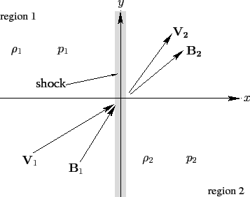
Here, $\rho_1$, $p_1$, $\mathbf{V}_1$, and $\mathbf{B}_1$ are the downstream mass density, pressure, velocity, and magnetic field, respectively, whereas $\rho_2$, $p_2$, $\mathbf{V}_2$, and $\mathbf{B}_2$ are the corresponding upstream quantities.

The basic RH relations are listed in MHD shocks.

There are 6 scalar equations and 12 scalar variables ($\rho, v_t, v_n, p, B_t, B_n$ for both upstream and downstream). This means that given all the upstream quantities, the downstream values are deterministic.

The categories are shown in the following table. We refer the changes of the downstream compared with the upstream.

Type	Particle Transport	$\rho$	$\mathbf{v}$	$p$	$\mathbf{B}$	T
Contact	No	$\pm$	continuous	continuous	continuous	$\pm$
Tangential[3]	No	$\pm$	continuous	$\pm$	$B_n$ = 0	$\pm$
Slow	Yes	+	-	+	$B_t$ -	+
Intermediate[4]	No	continuous	$\pm$	$\pm$	rotation	$\pm$
Fast[5]	Yes	+	-	+	$B_t$ +	+

[3]

The Earth's magnetopause is generally a tangential discontinuity. When there is no flux rope been generated, the magnetopause can be treated as the surface of pressure balance between magnetic pressure, ram pressure and thermal pressure. However, when reconnection triggers flux rope generation, it may become a rotational discontinuity.

[4]	A special case is called rotational discontinuity. All are isentropic. The tangential components of $\mathbf{B}$ and $\mathbf{v}$ must rotate together. Their existence are still a matter of debate.

[5]	The Earth's bow shock is a fast mode shock.

Parallel Shock

The first special case is the so-called parallel shock in which both the upstream and downstream plasma flows are parallel to the magnetic field, as well as perpendicular to the shock front.

As you may have probably guessed, a parallel shock is unaffected by the presence of a magnetic field. In fact, this type of shock is identical to that which occurs in neutral fluids, and is, therefore, usually called a hydrodynamic shock.

Is there a preferential direction from the upstream to the downstream? Yes, with the additional physics principle of the second law of thermodynamics. This law states that the entropy of a closed system can spontaneously increase, but can never spontaneously decrease. Now, in general, the entropy per particle is different on either side of a hydrodynamic shock front. Accordingly, the second law of thermodynamics mandates that the downstream entropy must exceed the upstream entropy, so as to ensure that the shock generates a net increase, rather than a net decrease, in the overall entropy of the system, as the plasma flows through it.

The (suitably normalized) entropy per particle of an ideal plasma takes the form

$S = ln(\frac{p}{\rho^\gamma}).$

After some derivations, it follows that the second law of thermodynamics requires hydrodynamic shocks to be compressive: i.e., $r>1$, where $r$ is the density jump ratio $\rho_2 / \rho_1$. In other words, the plasma density must always increase when a shock front is crossed in the direction of the relative plasma flow. It turns out that this is a general rule which applies to all three types of MHD shock. In the shock rest frame, the shock is associated with an irreversible (since the entropy suddenly increases) transition from supersonic to subsonic flow.

Note that $r\equiv \rho_2/\rho_1\rightarrow (\gamma+1)/(\gamma-1)$, whereas $R\equiv p_2/p_1\rightarrow\infty$, in the limit $M_1\rightarrow \infty$. In other words, as the shock strength increases, the compression ratio, $r$, asymptotes to a finite value, whereas the pressure ratio, $P$, increases without limit. For a conventional plasma with $\gamma=5/3$, the limiting value of the compression ratio is 4: i.e., the downstream density can never be more than four times the upstream density. We conclude that, in the strong shock limit, $M_1\gg 1$, the large jump in the plasma pressure across the shock front must be predominately a consequence of a large jump in the plasma temperature, rather than the plasma density.

Perpendicular Shock

The second special case is the so-called perpendicular shock in which both the upstream and downstream plasma flows are perpendicular to the magnetic field, as well as the shock front.

Going through the derivations, we find that the condition for the existence of a perpendicular shock is that the relative upstream plasma velocity must be greater than the upstream fast wave velocity,

$\mathbf{V}_1^2 > \mathbf{V}_{s1}^2 + \mathbf{V}_{A1}^2$

Incidentally, it is easily demonstrated that if this is the case then the downstream plasma velocity is less than the downstream fast wave velocity. We can also deduce that, in a stationary plasma, a perpendicular shock propagates across the magnetic field with a velocity which exceeds the fast wave velocity.

In the strong shock limit, $M_1\gg 1$, a strong perpendicular shock is very similar to a strong hydrodynamic shock (except that the former shock propagates perpendicular, whereas the latter shock propagates parallel, to the magnetic field). In particular, just like a hydrodynamic shock, a perpendicular shock cannot compress the density by more than a factor $(\gamma+1)/(\gamma-1)$. However, according to the RH jump conditions, a perpendicular shock compresses the magnetic field by the same factor that it compresses the plasma density. It follows that there is also an upper limit to the factor by which a perpendicular shock can compress the magnetic field.

Oblique Shock

Let us now consider the general case in which the plasma velocities and the magnetic fields on each side of the shock are neither parallel nor perpendicular to the shock front. It is convenient to transform into the so-called de Hoffmann-Teller frame in which $|\mathbf{V}_1\times \mathbf{B}_1|=0$, or

$V_{x1}B_{y1} - V_{y1}B_{x1} = 0.$

In other words, it is convenient to transform to a frame which moves at the local $\mathbf{E}\times\mathbf{B}$ velocity of the plasma.[HT_frame] It immediately follows from the jump condition of the magnetic convection equation that

$V_{x2}B_{y2} - V_{y2}B_{x2} = 0,$

or $|\mathbf{V}_2\times \mathbf{B}_2|=0$. Thus, in the de Hoffmann-Teller frame, the upstream plasma flow is parallel to the upstream magnetic field, and the downstream plasma flow is also parallel to the downstream magnetic field.

As before, the second law of thermodynamics mandates that $r>1$.

Let us first consider the weak shock limit $r\rightarrow 1$. In this case, it is easily seen that the three roots of the shock adiabatic reduce to the slow, intermediate (or Shear-Alfvén), and fast waves, respectively, propagating in the normal direction to the shock front. We conclude that slow, intermediate, and fast MHD shocks degenerate into the associated MHD waves in the limit of small shock amplitude. Conversely, we can think of the various MHD shocks as nonlinear versions of the associated MHD waves.

We can conclude that (in the de Hoffmann-Teller frame) fast shocks refract the magnetic field and plasma flow (recall that they are parallel in our adopted frame of the reference) away from the normal to the shock front, whereas slow shocks refract these quantities toward the normal. Moreover, the tangential magnetic field and plasma flow generally reverse across an intermediate shock front.

Let us now consider the strong shock limit, $v_1^{\,2}\gg 1$. There is only one root for the shock adiabatic, which is a fast shock. The fact that there is only one real root suggests that there exists a critical shock strength above which the slow and intermediate shock solutions cease to exist. (In fact, they merge and annihilate one another.) In other words, there is a limit to the strength of a slow or an intermediate shock. On the other hand, there is no limit to the strength of a fast shock. Note, however, that the plasma density and tangential magnetic field cannot be compressed by more than a factor $(\gamma+1)/(\gamma-1)$ by any type of MHD shock.

Consider the special case $\theta_1=0$ in which both the plasma flow and the magnetic field are normal to the shock front. There we have "switch-on" and "switch-off" shocks which refer to the generation and elimination of tangential components of the plasma flow and the magnetic field.

Consider another special case $\theta_1=\pi/2$. We have only one root that corresponds to the fast shock, except that there is no plasma flow across the shock front in this case.[HT_transition] The fact that the two other roots are zero indicates that, like the corresponding MHD waves, slow and intermediate MHD shocks do not propagate perpendicular to the magnetic field.

Double Adiabatic Theory

The classical approach by Chew, Goldberger, and Low CGL utilizes the MHD framework by assuming isotropic distributions parallel and perpendicular to the magnetic field, which results in scalar pressures on the two sides of the shock.

When we shift to the MHD with anisotropic pressure tensor

$P_{ij} = p_\perp \delta_{ij} + (p_\parallel - p_\perp)B_i B_j / B^2,$

where $p_\perp$ and $p_\parallel$ are the pressures perpendicular and parallel w.r.t. the magnetic field, respectively. For the strong magnetic field approximation, the two pressures are related to the plasma density and the magnetic field strength by two adiabatic equations,

$\begin{aligned} \frac{d}{dt}\Big( \frac{p_\parallel B^2}{\rho^3} \Big) &= 0, \\ \frac{d}{dt}\Big( \frac{p_\perp}{\rho B} \Big) &= 0. \end{aligned}$

This is also known as the double adiabatic theory,^[6] which is also what many people remember to be the key conclusion from the CGL theory. Here I want to emphasize the meaning of adiabatic again: this assumes zero heat flux. If the system is not adiabatic, the conservation of these two quantities related to the parallel and perpendicular pressure is no longer valid, and additional terms may come into play such as the stochastic heating.

[6]	These are constants at a fixed location in time: it is not correct to apply these across the shock!

The general jump conditions for discontinuities in a collisionless anisotropic magnetoplasma in the CGL approximation were derived by Abraham-Shrauner 1967.

The general jump conditions for an anisotropic plasma are given by Hudson 1970

$\begin{aligned} [\![ \rho v_n ]\!] &= 0, \\ [\![ v_n\mathbf{B}_t - \mathbf{v}_t B_n ]\!] &= 0, \\ [\![ p_\perp + (p_\parallel - p_\perp)\frac{B_n^2}{B^2} + \frac{B_t^2}{8\pi} + \rho v_n^2 ]\!] &= 0, \\ [\![ \frac{B_n \mathbf{B}_t}{4\pi}\big( \frac{4\pi(p_\parallel - p_\perp)}{B^2} - 1 \big) +\rho v_n \mathbf{v}_t ]\!] &= 0, \\ [\![ \rho v_n\big( \frac{\epsilon}{\rho} + \frac{v^2}{2} + \frac{p_\perp}{\rho} + \frac{B_t^2}{4\pi \rho} \big) + \frac{B_n^2 v_n}{B^2}&(p_\parallel - p_\perp) \\ - \frac{\mathbf{B}_t\cdot\mathbf{v}_t B_n}{4\pi}\big( 1 - \frac{4\pi(p_\parallel - p_\perp)}{B^2} \big) ]\!] &= 0, \\ [\![ B_n ]\!] &= 0, \end{aligned}$

where ρ is the mass density, v and B are the velocity and magnetic field strength. Subscripts t and n indicate tangential and normal components with respect to the discontinuity. Quantities $p_\perp$ and $p_\parallel$ are the elements of the plasma pressure tensor perpendicular and parallel with respect to the magnetic field. Quantity $\epsilon$ is the internal energy, $\epsilon = p_\perp + p_\parallel/2$, and $[\![ Q ]\!] = Q_2 - Q_1$, where subscripts 1 and 2 signify the quantity upstream and downstream of the discontinuity. These equations refer to the conservation of physical quantities, i.e. the mass flux, the tangential component of the electric field, the normal and tangential components of the momentum flux, the energy flux, and, finally, the normal component of the magnetic field. To solve the jump equations for anisotropic plasma conditions upstream and downstream of the shock, one has to use an additional equation, since the set of equations is underdetermined. One common choice is the magnetic field/density jump ratio.

The following derivations originate from Erkaev+ 2001. Let us introduce two dimensionless parameters, $A_s$ and $A_m$, which are determined for upstream conditions as

$\begin{aligned} A_s &= \frac{p_{\perp 1}}{\rho_1 v_1^2} \\ A_m &= \frac{1}{M_A^2}, \end{aligned}$

where $M_A$ is the upstream Alfvén Mach number. For common solar wind conditions, both of these parameters are quite small ($\sim 0.01$).

For shocks, the tangential components of the electric and magnetic fields are coplanar.^[7] Thus, the components of the magnetic field upstream of the shock are given as $B_{n1} = B_1 \cos\gamma$ and $B_{t1} = B_1 \sin\gamma$, where γ is the angle between the magnetic field vector and the vector $\widehat{n}$ normal to the discontinuity. Similarly, the components of the bulk velocity upstream of the shock are chosen as $v_{n1} = v_1 \cos\alpha$ and $v_{t1} = B_1 \sin\alpha$, where α the angle between the bulk velocity and the normal component of the velocity. Furthermore, a parameter λ is used to denote the pressure anisotropy

$\lambda = p_\perp / p_\parallel,$

and another parameter x is used to denote the ratio of density

$x \equiv \frac{\rho_2}{\rho_1} = \frac{v_{n1}}{v_{n2}}.$

[7]	I still don't fully get it...

Perpendicular Shock

For a perpendicular shock, $B_n = 0$, we have the conservation relations reduce to

$\begin{aligned} [\![ \rho v_n ]\!] &= 0, \\ [\![ v_n\mathbf{B}_t ]\!] &= 0, \\ [\![ p_\perp + \frac{B_t^2}{8\pi} + \rho v_n^2 ]\!] &= 0, \\ [\![ \rho v_n \mathbf{v}_t ]\!] &= 0, \\ [\![ \rho v_n\big( \frac{\epsilon}{\rho} + \frac{v^2}{2} + \frac{p_\perp}{\rho} + \frac{B_t^2}{4\pi \rho} \big) ]\!] &= 0. \end{aligned}$

The quantities downstream of the discontinuity are

$\begin{aligned} B_{t2} &= x B_{t1}, \\ v_{t2} &= v_{t1}, \\ p_{\perp 2} &= p_{\perp 1} + \frac{B_{t1}^2}{8\pi}(1-x^2) + \rho_1 v_{n1}^2\big( 1 - \frac{1}{x} \big). \end{aligned}$

Substituting these into the energy equation leads to

$\begin{aligned} 2 \lambda_1(3\lambda_2 +1)y^3 − \lambda_1(4\lambda_2 +1)(2A_S + A_M +2)y^2 \\ + \lambda_2[2\lambda_1(4A_S + 1 + 2A_M ) + 2A_S ]y + A_M \lambda_1 = 0, \end{aligned}$

where $y = 1/x$.

Now we can do some simple estimations. Assume we have isotropic upstream solar wind with $n = 2 \textrm{amu/cc}$, $\mathbf{v} = [600, 0, 0] \textrm{km/s}$, $\mathbf{B} = [0, 0, -5] \textrm{nT}$ in GSM coordinates, and $T = 5\times 10^5 \textrm{K}$. We want to estimate the downstream anisotropy given a density/tangential magnetic field jump of 3.

using Vlasiator: kB, μ₀, mᵢ

n1 = 2e6  # [m^3]
v1 = 6e5  # [m/s]
B1 = 5e-9 # [T]
T1 = 5e5  # [K]
λ1 = 1.0

As = kB * T1 / (mᵢ * v1^2)        # 0.011
Am = B1^2 / (μ₀ * mᵢ * n1 * v1^2) # 0.016

x = 3     # downstream/upstream jump density ratio
y = 1 / x

λ2 = (-2λ1*y^3 + λ1*(2As+Am+2)*y^2 - Am*λ1) /
   (6λ1*y^3 - 4λ1*(2As+Am+2)*y^2 + (2λ1*(4As+1+2Am)+2As)*y)

@show λ2

which shows $\lambda_2 \simeq 3.19$.

In Vlasiator 2D southward IMF equatorial run I get 15 in a large area with spatial resolution 300 km downstream near the shock, which is much larger than this. I later realized that this indicates that the run is problematic, because the periodic condition in the out-of-plane z direction, which is also the parallel direction, prohibits any parallel heating. This in turn causes unphysical anisotropy values in the downstream region.

In Vlasiator 2D southward IMF meridional run I get over 10 in a narraw region downstream of the shock, but for most part of the magnetosheath, the value is between 1 to 5, except the region near the magnetopause where again we have values over 10.

Another thing to note is that, if you set the jump ratio to 4 in the above calculations, the downstream anisotropy will become 0.6. This indicates that under this set of upstream conditions, the jump ratio shall never be close to 4 if you want anisotropy value > 1!

Parallel Shock

Parallel shocks are more special in that the magnetic field strength remains unchanged so the equations effectively describe pure gasdynamic solutions. Kuznetsov & A.I.Osin, 2018 presents a simplified solution in a 1D parallel shock case with parallel and perpendicular thermal energy heat fluxes $S_\parallel$ and $S_\perp$ included. Note again the original CGL theory assumes 0 heat fluxes.

Location of Shock

In the observation comparison paper Slavin and Holzer, 1981 for quasi-perpendicular shocks, they concluded that the variations in shock stand-off distance and shape are ordered by the sonic Mach number and not other Mach numbers involve magnetic field. In other words, they think the bow shock is a gasdynamic structure.

However, even in neutral fluid theory, the determination of shock location as well as shape is still a research problem. Imagine the simplest scenario where there is a static ball in the air with infinite mass. Assuming purely homogenous air with known density, velocity and pressure in the upstream, can you tell me the exact location of shock stand-off distance with pen and paper?

On top of that, the introduction of EM field complicates the story. Especially in the case of a parallel shock, the plasmas get "shocked" both upstream and downstream, and the stand-off distance of the shock may not be a single point theoretically. In some sense, normal magnetic field to the boundary "thickens" the shock front.

Anisotropy in the Solar Wind

Observationally, Pioneer 6 showed that the ion temperature anisotropy in the solar wind at 1AU generally has $T_\parallel > T_\perp$^[8]. It may possibly be explained by the conservation of the 1st adiabatic invariant Scarf+, 1967^[9].

[8]	There are 3 interesting discoveries from Pioneer 6 ARC plasma measurements:

1. high fluctuations of flow velocity outside the solar ecliptic plane;

2. anisotropic ion thermal distribution ($T_\parallel / T_\perp \sim [2,5]$);

3. presence of a 3rd species, helium, from charge-to-mass ratio analysis of the angular and energy distributions.

[9]	I love this old paper. The pioneers in our field did real physics.

The magnetic moment

$\mu = \frac{m v_\perp^2}{2B}$

is conserved as the collisionless solar wind flows outward from the sun. Near the solar equator the mean field magnitude declines with

$B_r(r) \simeq B_r(r_0)\Big( \frac{r_0}{r} \Big)^2$

and

$B_\phi(r) \simeq \frac{\Omega_r}{u(r)}B_r(r)$

from the Parker spiral solar wind model and $\Omega_r = 2.94\times 10^{-6}$ rad/s being the angular frequency of the rotation of the sun.

The adiabatic equation in the perpendicular direction indicates that the perpendicular thermal energy $\langle m v_\perp^2/2\rangle = k_B T_\perp$ declines with B. Assuming in the rest frame the distribution function is a bi-Maxwellian of the form

$f(v) = \Big( \frac{m}{2\pi} \Big)^{3/2}\frac{1}{k_B T_\perp (k_B T_\parallel)^{1/2}} \exp\Big( -\frac{mv_\perp^2}{2k_B T_\perp} -\frac{mv_\parallel^2}{2k_B T_\parallel} \Big),$

the conservation of the total thermal energy

$W = \int d^3v \frac{mv^2}{2}f(v)$

yields

$W = k_B T_\perp + k_B T_\parallel/2 = const.$

These allows us to evaluate the variations in $T_\perp$ and $T_\parallel$ originating from isotropic distribution on the surface of the sun. Starting from $T_\perp(0.3 AU) = T_\parallel(0.3 AU)\simeq 1.3\times 10^{5}\textrm{K}$, the predicted anisotropy at Earth can go beyond 20! Therefore in fact, the reasonable question to ask is why the actual solar wind anisotropy factor is so small.^[10]

[10]	This is new to me. Since I've been involved in the simulation reseach, we always apply isotropic distribution in the upstream solar wind condition, which I guess is primarily due to the fact that we are mostly using MHD. Should we now use more realistic distributions with the kinetic models?

Well, we know now when pressure anisotropy develops, two kinds of plasma instabilities can be triggered: firehose when $T_\perp < T_\parallel$ and mirror when $T_\perp > T_\parallel$. Further studies require kinetic theory to describe their behaviors.

On the other hand, the opposite case, $T_\perp > T_\parallel$, is also observed and believed to be related to local ion heating by macroscale compressions (e.g. high/low speed streams interaction) or plasma instabilities Barne+ 1975.

Here I list the mirror instability criterion as an additional relation to determine the pressure anisotropy downstream of the shock from the book Plasma instabilities and nonlinear effects by Hasegawa 1975,

$1 + \sum_{\textrm{species}} \beta_\perp \big( 1 - \frac{\beta_\perp}{\beta_\parallel} \big) < 0.$

Earth Bow Shock

Using data from the AMPTE/IRM spacecraft, Hill+ 1995 have shown that the double adiabatic equations do not hold in the magnetosheath. Moreover, the thermal behaviour of the magnetosheath is studied by Phan+ 1996 using WIND spacecraft data. They report that most parts of the magnetosheath are marginally mirror unstable.^[11]

[11]	WIND has electron observations and shows $T_{e\perp} / T_{e\parallel} \sim 1.3$ in the magnetosheath.