Testing

There exists some test funtionalities under the testpackages folder, but it is not good enough.

• Currently one can compare the output from one version of the code to another version, but obviously there are many problems with this approach. How can you guarantee the version you select generate the correct "reference" solutions?

• The shell scripts are written for specific machines, but none of them are running on a regular basis.

• One has to do many extra work to create tests on a new machine.

• We cannot pick a specific test to run easily with one command.

To tackle these problems, I am thinking about redesign the whole test suites. The goal is to

• define reference solutions to compare with;

• create a flexible test list with make;

• test one thing at a time;

• introduce continuous integration (CI) to validate new development and changes.

There is a tool written in C++ called vlsvdiff that can be used to compare two VLSV files. This can be used to investigate the differences between files. For automated tests, it is enough to know that there are differences. The difficulties for VLSV file format result from the random writing order from MPI processes. If you are running with multiple MPI processes, you may get different SHA values out of the VLSV file even if the data are actually identical.

How to store the reference solutions? Well, they should be saved in a different repository to keep the main source repo clean. To compare results, more often than not we do not need the raw distribution values f: by not saving it we can save a lot of storage!

Comparing Differences

This is a big headache now. I get different results with different code versions on different platforms, even if there shouldn't be any.

1. There are two GCC optimization flags that will affect the results even on the same machine with slightly differernt code versions: -ffast-math, which boost the floating point operation performance by loosening the IEEE standard; -mavx, which turns on the avx instructions on the target machine. I can understand the first, but not the second one. Both flags have influence on the speed beyond -O3, which are about 10%.

2. Even if I turn off all the optimization flags, there are still differences running on different machines for multiple tests, e.g. acctest_1_maxw_500k_30kms_1deg. Among all the variables being saved there, the largest difference comes from populations_vg_rho_loss_adjust, which records the sparse distribution dropping/adding. I don't have any idea how this can happen: maybe the values are so small, and the round-off errors accumulate with timesteps?

Demo

Under the testpackage folder:

make

runs all the listed tests in Makefile.

make TESTS=flowthrough

runs a specific test.

It would be nice to save the test log somewhere, but for now just ignore it. Also vlsvdiff can substitute julia for comparing differences.

Tests

Some tests are borrowed from MHD-EPIC. We choose 3 reference values: $n_0=10^6\,\mathrm{m}^{-3}$, $B_0 = 10^{-8}\,\mathrm{T}$, $m_0=m_i$. All the other conversion factors from dimensionless to SI can be derived:

• lRef: 2.28e5 [m]

• tRef: 1.04 [s]

• vRef: 2.18e4 [m/s]

• nRef: 1e6 [#]

• TRef: 5.76e6 [K]

• PRef: 7.96e-11 [Pa]

• BRef: 1e-8 [T]

The length scale is the ion inertial length, the time scale is the gyro-period, and the velocity scale is the Alfvén speed.

To make sure the velocity space is refined as much as possible, we need to check the ratio between thermal speed and the vspace parameters. Based on empirical tests, the maximum vspace extent shall be $\sim 7 V_\mathrm{th} = 7\sqrt{\gamma p_0/\rho_0}$ with $V_\mathrm{th}/dv \sim 20$ with 80 vblocks (320 vcells) if the VDF threshold is set to $10^{-20}$.

In principle the choice of basic reference values should not effect the numerical results. As a referece, the single precision epsilon is $\epsilon=1.1920929f-7$, and the double precision epsilon is $\epsilon=2.220446049250313e-16$. Since Vlasov-Maxwell model does not suffer from the statistical noise issue as in PIC, we shall be able to test with smaller perturbations compared with typical PIC values.

Free stream test

Everything is uniform, which means nothing should change. Because of the existence of magnetic field, the rotation in the velocity space may have a detectable numerical effect.

$\gamma = 5/3$.

Variable	Background	Background (SI)
$\rho$	$1.0$	$1\times 10^6$
$u_x$	$0.0$	$0.0$
$u_y$	$0.0$	$0.0$
$u_z$	$0.0$	$0.0$
$p$	$1/\gamma=0.6$	$2.3873241463784306e-13$
$B_x$	$1.0$	$1\times 10^{-9}$
$B_y$	$\sqrt{2}$	$1.4142135\times 10^{-9}$
$B_z$	$0.5$	$0.5\times 10^{-9}$

• Single precision VDF:

  • Number density decreases by $2.5\times 10^{-7}$. The absolute error is on the order of single precision $\epsilon$.

  • Velocity changes from $0$ to $\sim\mathcal{O}(1)\,\mathrm{m/s}$. Not sure is this is ok.

  • Magnetic field keeps the initial values, which is good.

• Double precision VDF:

  • Number density error is below single precision $\epsilon$.

  • Velocity changes from $0$ to $\sim\mathcal{O}(10^{-6})\,\mathrm{m/s}$. I would say this is perfectly fine.

  • Magnetic field keeps the initial values, which is good.

Linear waves test

The waves are propagating in an oblique direction so as to check grid effects.

The results are really sensitive to the perturbation magnitude $A$. If $A=10^{-3}$, single and double precision results are almost identical; if $A=10^{-6}$, the single precision results are completely off while the double precision results at least still maintain the wave-like pattern. I found $A=10^{-4}$ as roughly when the single and double precision results differ.

The moments are very sensitive to the velocity grid resolutions as well as extent. With double precision VDFs, the initial condition follows the analytical solution well even at $A=10^{-6}$; with single precision VDFs, the initial condition has observable errors at $A=10^{-6}$ and even larger errors at larger $A$.

Double precision VDF runs are in general much better. Depending on the velocity space resolutions, the single precision VDF may not even has a average value of 0 velocity even if we set it to. Double precision does not suffer from this issue.

If the so-called "diffusive E" term is turned off in Vlasiator (by default it's on and 2nd order), the results are worse.

Alfvén wave

This test involves the propagation of Alfvén waves and whistler waves. The Alfvén/whistler waves have variations in the transverse components of the magnetic field and the velocity. The longitudinal components, the density and the pressure are not perturbed. The following solution of the Hall MHD equations describes a right-hand polarized Alfvén/whistler wave propagating in the $+x$-direction:

$$\begin{aligned} u_y &= -\delta u\cos(kx-\omega t) \\ u_z &= +\delta u\sin(kx-\omega t) \\ B_y &= +\delta B\cos(kx-\omega t) \\ B_z &= -\delta B\sin(kx-\omega t) \end{aligned}$$

where the magnetic and velocity perturbations are related as

$$\frac{\delta u}{\delta B} = \frac{B_x}{v_\mathrm{ph}\rho}$$

and the phase speed is

$$v_\mathrm{ph,A} = \frac{\omega}{k} = \frac{B_x}{\sqrt{\mu_0\rho}}$$

At larger k, Alfvén waves evolve into whistler waves, and the phase speed then depends on k:

$$v_\mathrm{ph,W} = \frac{\omega}{k} = \frac{W}{2} + \sqrt{\frac{B_x^2}{\mu_0\rho} + \frac{W^2}{4}},\quad W=\frac{m}{e}\frac{kB_x}{\mu_0\rho}$$

We set wavelength $\lambda=2\pi/k=32$ and the initial conditions as follows:

Variable	Background	Perturbations
$\rho$	$1.0$	$0.0$
$u_x$	$0.0$	$0.0$
$u_y$	$0.0$	$0.002$
$u_z$	$0.0$	$0.002$
$p$	$5.12\times 10^{-4}$	$0.0$
$B_x$	$0.2$	$0.0$
$B_y$	$0.0$	$0.002$
$B_z$	$0.0$	$0.002$

$v_W=0.22059$ which is about 10% faster than the Alfvén speed $V_A=0.2$, therefore the Hall term is small but not negligible at this wavelength. $\beta = 0.02$, so this is really in the cold plasma limit.

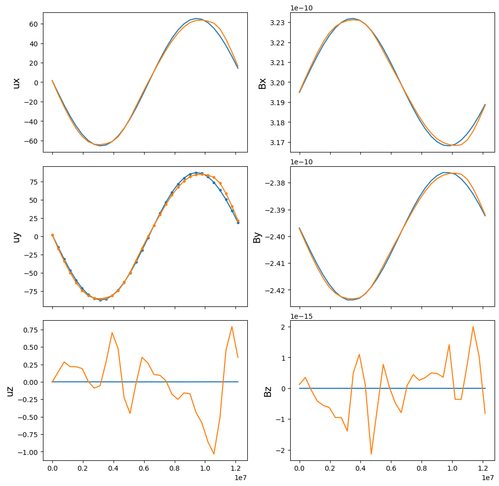
First we switch off the Hall term and check the Alfvén wave in Figure 1.

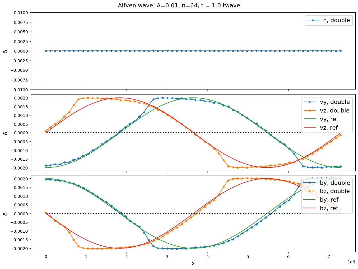
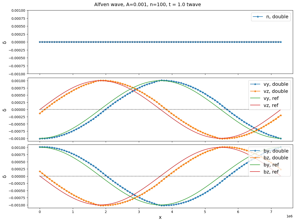
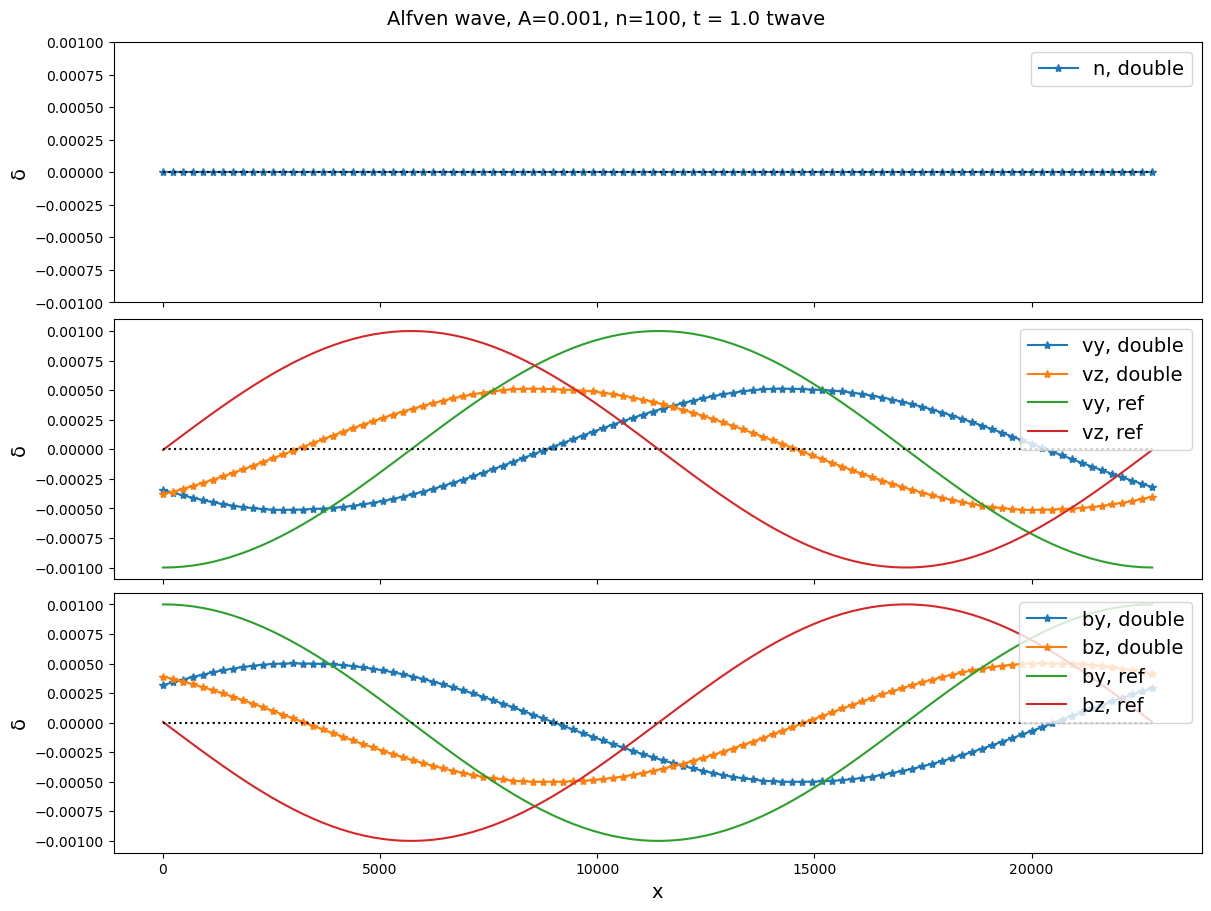
We see that the cold Alfvén wave after one period grows bumps trailing the peaks and troughs. This is associated with some tiny perturbations at the same locations for $\rho, u_x$ and $B_x$. After four periods, it becomes more discontinuous, but the amplitude does not grow. This does not seem like the usual wave steepening effect. Changing wavelength ($\lambda=32,1,0.1$) does not modify the behaviors. However, if we increase the thermal pressure to make $\beta\sim 1$, changing wavelength does generate significant differences, as shown in Figure 2 and 3.

Next we switch on the Hall term and check the whistler wave in Figure 4.

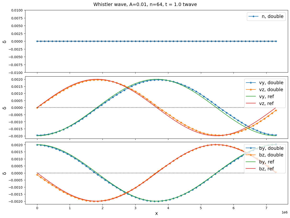
Interestingly, now even in the cold plasma limit we do not see the strange bumps. An observable change in the run log is that subcycling is now taking place: it take 29 subcycles instead of only 1-3 in the pure Alfvén wave test. But luckily we do not see any numerical instabilities. So a conclusion from the Alfvén/whistler test is that the Hall term is necessary even for the Alfvén wave in a hybrid model; without it we always see some distortions of the wave profile. The real reason might be that the time step taken in the field solver for just the convection term is too large.

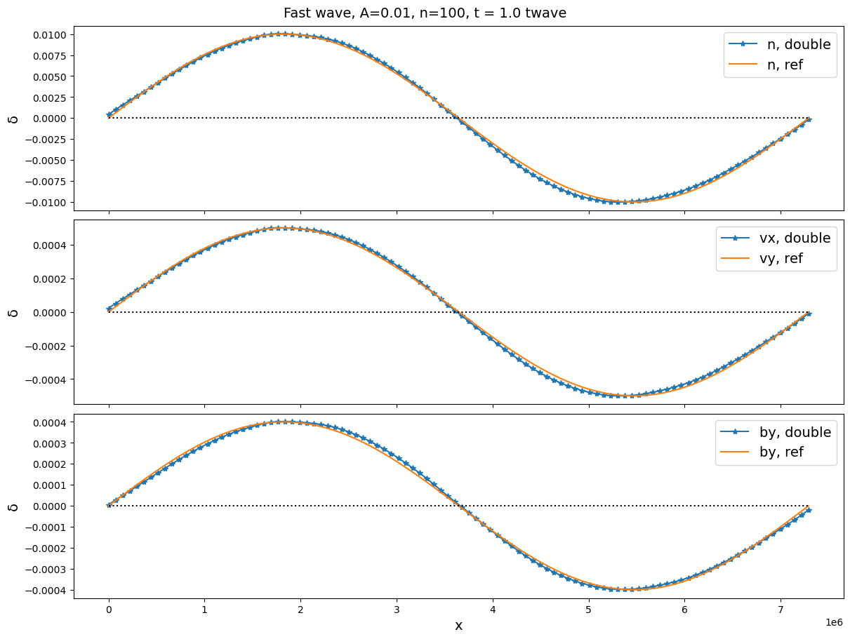
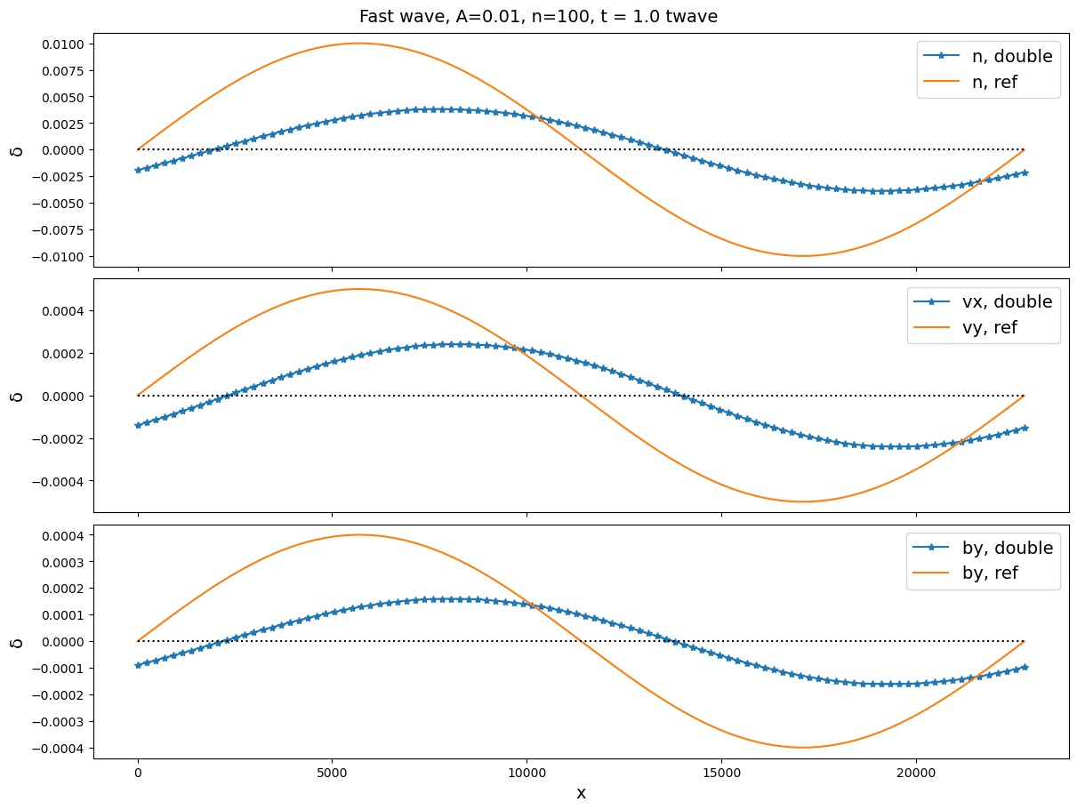
Fast wave

Classical fast wave assumes isotropy. In the kinetic description, the parallel and perpendicular pressures vary differently in the collisionless plasma even if the unperturbed plasma has isotropic pressure. The isotropic MHD solutions are not valid in models like anisotropic MHD, hybrid, or PIC.

The following equations are an exact solution of the anisotropic MHD equations

$$\begin{aligned} \rho &= \rho_0\left[ 1 + \delta\sin(kx-\omega t) \right] \\ u_x &= V_f \delta\sin(kx-\omega t) \\ u_y &= 0 \\ u_z &= 0 \\ p &= p_0\left[ 1 + \gamma\delta\sin(kx-\omega t) \right] \\ p_\parallel &= p_0\left[ 1 + \delta\sin(kx-\omega t) \right] \\ B_x &= 0 \\ B_y &= B_0 \left(1+\delta\sin(kx-\omega t)\right) \\ B_z &= 0 \end{aligned}$$

where $p = \frac{p_\parallel + 2p_\perp}{3}$ and

$$V_f = \frac{\omega}{k} = \sqrt{\frac{B_0^2 + 2 p_0}{\rho_0}}$$

is the propagation speed of the fast wave moving perpendicular relative to the magnetic field direction. Note that $p$ and $p_\parallel$ have different wave amplitudes, i.e. this solution is different from the isotropic (collisional) fast wave. Also note the $2p_0$ (actually $2p_\perp$) term instead of the usual $\gamma p$ term in the phase speed.

The initial conditions are set as following ($\rho_0 = 1, p_0 = 4.5\times 10^{-4}, B_0 = 0.04, \delta=0.01$):

Variable	Background	Perturbations
$\rho$	$\rho_0$	$\delta$
$u_x$	$0.0$	$V_f*\delta$
$u_y$	$0.0$	$0.0$
$u_z$	$0.0$	$0.0$
$p$	$p_0$	$p_0\gamma\delta$
$p_\parallel$	$p_0$	$p_0\delta$
$B_x$	$0.0$	$0.0$
$B_y$	$B_0$	$B_0\delta$
$B_z$	$0.0$	$0.0$

For the parameters listed here, $r_L / d_i = 0.68$. The results are shown in Figure 5 and 6. We can clealy see the strong damping and modification of wave speeds at a small wavelength compared with the gyroradius.

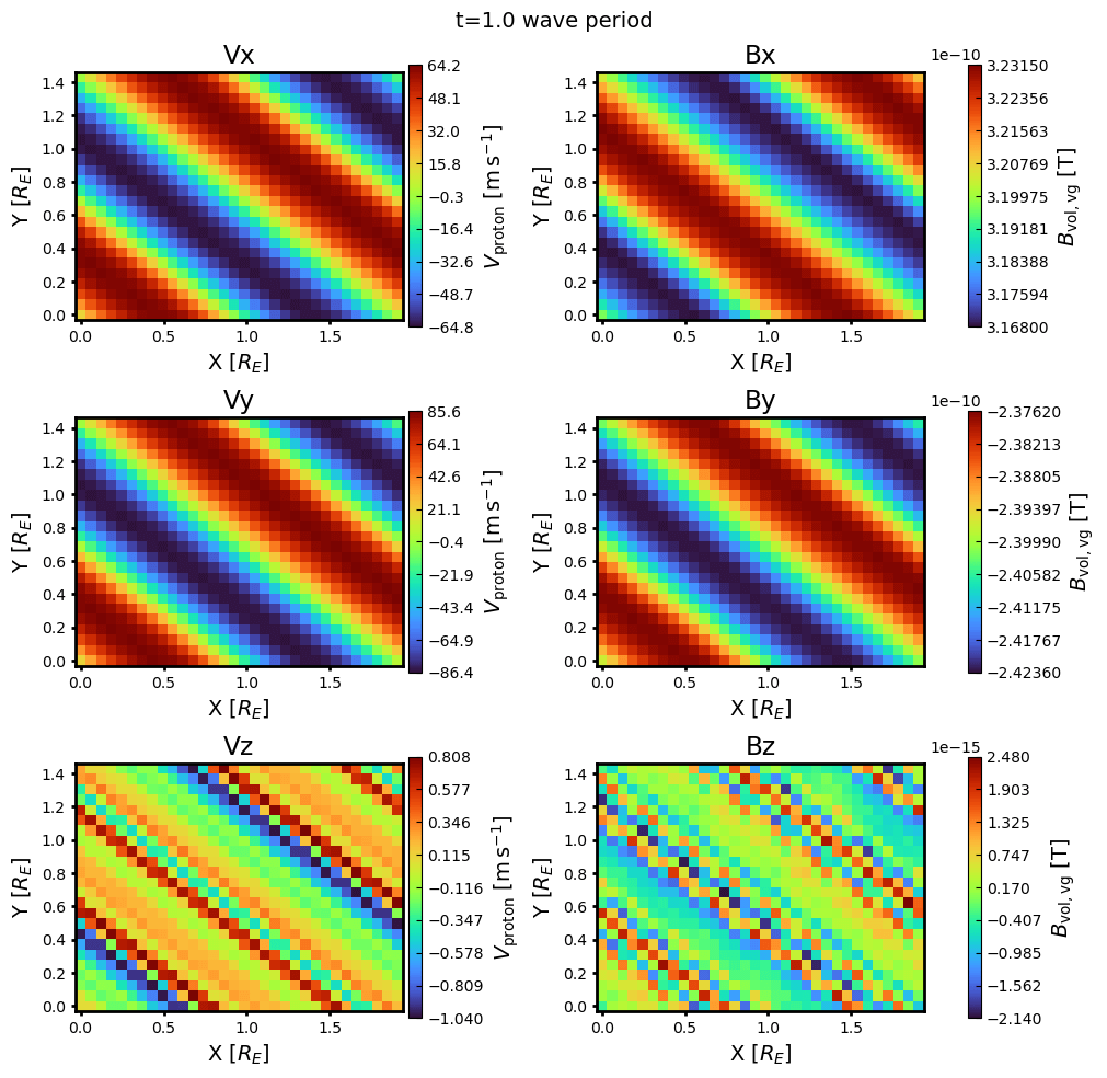
As a 2D setup, we rotate the whole problem with angle $\alpha=atan(-3/4)$ with respect to $+x$. The results are shown in Figure 7 and 8.

Slow wave

Slow wave test is tricky, in that slow wave does not propagate perpendicular to the magnetic field. If we simply modify the anisotropic fast wave test parameters, we would expect a zero phase speed slow wave with anti-correlated magnetic pressure and thermal pressure perturbations. I have not yet designed a proper set of parameters for slow waves.

We are unlikely to hit the mirror mode instability criterion

$$\left(\frac{p_\perp}{p_\parallel} - 1\right)\beta_\perp > 1$$

but this is something we need to check as well. There are specific tests for checking pressure anisotropic instabilities.

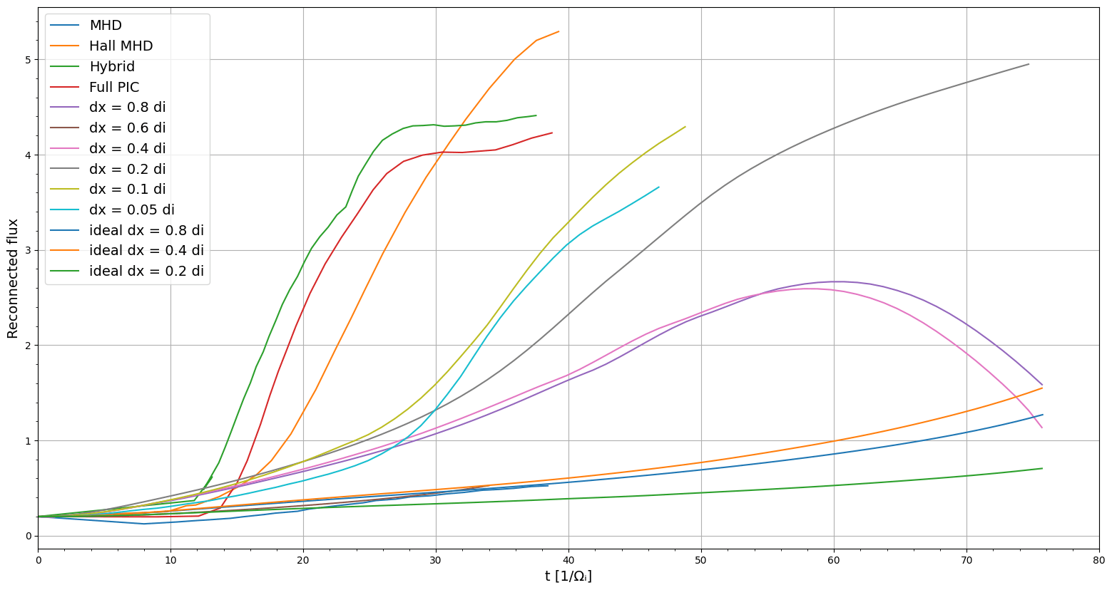
GEM Challenge

The GEM reconnection test is performed using Project Harris. The 2D colored contour of density overplotted with magnetic field lines are shown in Figure 9.

The normalized reconnection rates are shown in Figure 8. The points for MHD, Hall MHD, hybrid and full PIC are extracted from Figure 1 in Birn+ 2001. Without the Hall term, the reconnection rate is significantly lower than others and is comparable with ideal MHD. Resolving the ion inertial length is also important to get fast reconnection rates. The reason we have a delayed onset for Vlasiator compared with PIC may be due to the fact that we have smaller noises (suggested from Takuma Nakamura).