Vlasiator

Vlasiator is a numerical model for collisionless ion-kinetic plasma physics. Urs Ganse gave a lecture of Vlasiator for ISSS14.

Features

Vlasov solvers in higher dimensions are known to be slow. But how slow it is? 3D Earth: 1 week of running = 6 million cpu hours?

One restart file for 3D Earth now is typically ~2TB.

• semi-Lagrangian Vlasov solver for ions

• massless fluid treatment of electrons

• 3D mesh refinement in Cartesian boxes

• Up to isotropic $\nabla P_e$ term in the Ohm's law when solving for the electric field?

Overview

The fundamental description of charged particle motion in an electromagnetic field is given by the Vlasov equation

$$\frac{\partial f_\alpha}{\partial t} + \mathbf{v}_\alpha\frac{\partial f_\alpha}{\partial \mathbf{r}_\alpha} + \mathbf{a}_\alpha\cdot \frac{\partial f_\alpha}{\partial \mathbf{v}_\alpha} = 0,$$

where $\mathbf{r}_\alpha$ and $\mathbf{v}_\alpha$ are the spatial and velocity coordinates, $f(\mathbf{r},\mathbf{v},t)$ is the six-dimensional phase-space density of a particle species with mass m and charge q, and acceleration $\mathbf{a}$ is given by the Lorentz force

$$\mathbf{a}_\alpha = \frac{q_\alpha}{m_\alpha}(\mathbf{E}+\mathbf{v}_\alpha\times\mathbf{B}),$$

where $\mathbf{E}$ and $\mathbf{B}$ are the electric and magnetic field, respectively.

The bulk parameters of the plasma, such as the ion density $n_\alpha$ and velocity $\mathbf{u}_\alpha$, are obtained as velocity moments of the ion velocity distribution function

$$n_\alpha = \int d^3 v f(\mathbf{r},\mathbf{v},t),$$ $$\mathbf{u}_\alpha = \int d^3 v \mathbf{v}f(\mathbf{r},\mathbf{v},t).$$

The magnetic field is updated using Faraday's law:

$$\nabla \times \mathbf{E}_{\text{Ohm}} = -\frac{\partial \mathbf{B}}{\partial t},$$

and the system is closed by Ohm's law giving the electric field $\mathbf{E}_{\text{Ohm}}$. Depending on the order of approximation, the simplest one only takes the convection electric field

$$\mathbf{E}_\text{Ohm} = -\mathbf{u}_\alpha \times\mathbf{B},$$

where $\mathbf{u}_i$ is the ion bulk velocity given previously. The electric field exerted on the ion is given by

$$\mathbf{E}_\alpha = -\mathbf{u}_\alpha \times\mathbf{B} + \frac{1}{\rho_q}\mathbf{j}\times\mathbf{B}.$$

The second term on the right hand side is the Hall term, which must be included otherwise no bulk force is exerted on the ions. The total current density $\mathbf{j}$ is obtained from Ampère–Maxwell's law where the displacement current has been neglected:

$$\nabla\times\mathbf{B} = \mu_0 \mathbf{j}.$$

Vlasov solver

The kernal of the model is a Vlasov equation solver for the phase space distribution function $f(\mathbf{r},\mathbf{v},t)$. This is a scalar appeared in an advection equation in high dimension space, so basically we need to look for a scheme that can propagate a scalar in high dimension space accurately.

Finite volume method

The early versions of Vlasiator adopted a finite volume method for the Vlasov solver. The full 6D spatial and velocity space is discretized into ordinary and velocity cells. Each spatial cell contains the field variables ($\mathbf{B},\mathbf{E}$), which are stored on a staggered grid with $\mathbf{B}$ on the face centers and $\mathbf{E}$ on the edges. Each spatial cell also contains a 3D Cartesian velocity mesh where each velocity cell contains ths volume average $\tilde{f}$ of the distribution function over the ordinary space volume of the spatial cell, and the velocity space volume of the velocity mesh cell

$$\tilde{f} = \frac{1}{\Delta^3 r \Delta^3 v}\int_{cell} d^3r d^3 v f(\mathbf{r},\mathbf{v},t),$$

where $\Delta^3 r = \Delta x \Delta y \Delta z$ and $\Delta^3 v = \Delta v_x \Delta v_y \Delta v_z$ denote the phase space integration volumes, and $\Delta x$ e.t.c are the sizes of the cell in each dimension. The volume average $\tilde{f}$ is propagated forward in time by calculating fluxes at every cell face in each of the six dimensions. In the case of Vlasov's equation the spatial ($F_x, F_y, F_z$) and velocity ($F_{vx}, F_{vy}, F_{vz}$) fluxes take on particularly simple forms,

$$\mathbf{F}_\mathbf{r} = \mathbf{v}f,$$ $$\mathbf{F}_v = \frac{q}{m}\Big( \mathbf{v} - \mathbf{V}_i + \frac{1}{\mu_0 \rho_q}\nabla\times\mathbf{B} \Big)\times\mathbf{B}f.$$

$\mathbf{B}$ is a volume average calculated from face averages using divergence-free reconstruction polynomials given in Balsara+ (2009). The propagation of $\tilde{f}$ is given by

$$\tilde{f}(t+\Delta t) = \tilde{f}(t) - \sum_{i=x,y,z}\frac{\Delta t}{\Delta r_i}\big[ F_i(r_i+\Delta r_i) - F_i(r_i) \big] - \sum_{i=vx,vy,vz}\frac{\Delta t}{\Delta v_i}\big[ F_{vi}(v_i+\Delta v_i) - F_{vi}(v_i) \big].$$

By construction the FVM scheme here guarantees the conservation of mass except at the boundaries of the simulation domain. This is further split into the spatial translation $S_T$ and acceleration $S_A$ operators. Both operators propagate the distribution function with a $2^{nd}$ order accurate method based on solving 1D Riemann problems at the cell faces and applying flux limiters to suppress oscillations. Each cell face can contribute to the flux in up to 18 adjacent cells.

Here the monotonized central (MC) limiter (van Leer, 1977) has been used since it does not distort the shape of the original Maxwellian distribution. More aggressive limiters such as superbee or Sweby (Roe, 1986; Sweby, 1984) can reduce the diffusion more efficiently even for low velocity resolution but their applicability for kinetic plasma simulations is questionable as they tend to distort the shape by flattening the top and steepening the edges of the distribution function.

Strang (1968) splitting is used to propagate the distribution in time

$$\tilde{f}(t+N\Delta t) = \Big[ S_T(0.5 \Delta t) S_A(\Delta t) S_T(0.5\Delta t) \Big]^N \tilde{f}(0).$$

The leap-frog scheme is used for propagation. The algorithm is stable as long as the timestep fulfills the Courant–Friedrichs–Lewy (CFL) condition. The Courant number is for each dimension given by

$$C = \frac{u\Delta t}{\Delta s},$$

where $u$ corresponds to the velocity: $v_x$, $v_y$ and $v_z$ in ordinary space and $a_x$, $a_y$ and $a_z$ in velocity space. $\Delta s$ corresponds to the size of the simulation cell: $\Delta x$, $\Delta y$ and $\Delta z$ in ordinary space and $\Delta v_x$, $\Delta v_y$ and $\Delta v_z$ in velocity space.

In simulations with strong local fields leading to high acceleration, e.g., Earth's dipole magnetic field, the timestep is limited by the acceleration $S_A$ operator. To enable larger timesteps we split the propagation in velocity space into shorter substeps, where the length of each substep is set according to the CFL condition so that the Courant number of the substep is in the middle of the allowed range. The magnetic field is constant during the substepping, but the effective electric field does change as we recompute the bulk velocity $\mathbf{V}_i$ in Eq. (12) after each substep. By substepping the acceleration operator we can keep the global timestep reasonable, which minimizes the total number of timesteps in a simulation. The length of the substep is computed on a cell-by-cell basis, thus substepping only happens close to Earth in magnetospheric simulations. When we substep, the propagation of the distribution function is not $2^nd$ order accurate in time.

Semi-Lagrangian method

Why not continuing using the FV Vlasov solver?

• FVM has a CFL timestep limitation, where in the Vlasov equation is mostly constrained by the rotation in the acceleration term $\mathbf{v}\times\mathbf{B}$.

• For whatever reason numerical heating is significant, even in free-stream test. For example, a fixed-state solar wind propagating $10\,\text{R}_E$ from the upstream boundary to the bow shock would be heated drastically. (Note: this is still a problem even for SLM!)

Therefore after version 4 Vlasiator switched to a Semi-Lagrangian method. It has "semi" as prefix due to the fact that it is a mixture of Eulerian grid and Lagrangian method^[1]. The idea is that unknowns are still defined in a Eulerian grid, and to calculate the quantities at the next step n+1, we trace the control volume one step before at n and find the corresponding volume integrated value through an interpolation approach. Due to the conservation law, this is exactly the value we seek at the next timestep. As of Vlasiator 5.0, the semi-Lagrangian method being used is SLICE3D.

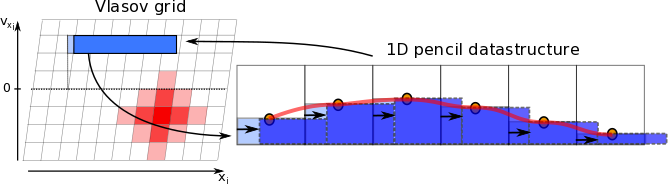
In the implementation, the 6 phase space dimensions (3 regular space, 3 velocity space dimensions, i.e. "3D3V") are treated independently. This is known as the Strang-splitting approach. There are three terms in Vlasov equation: the time-derivative, the spatial derivative (which is called translation), and the velocity derivative (which is called acceleration). Translation and acceleration are performed consecutively. For each dimension, transport in the $(x_i,v_{xi})$ subspace forms a linear shear of the distribution, as illustrated in Figure 1.

In a similar way, the acceleration update profits from the structure of the electromagnetic forces acting on the particles. In the nonrelativistic Vlasov equation, the action of the Lorentz force $\mathbf{F}_l = q_\alpha (\mathbf{E}+\mathbf{v}\times\mathbf{B})$ transforms the phase space distribution inside one simulation time step $\Delta t$ like a solid rotator in velocity space: the magnetic field causes a gyration of the distribution function by the Larmor motion

$$\frac{\partial \mathbf{v}}{\partial t} = q_\alpha \mathbf{v}\times\mathbf{B}$$

while the electric field causes (1) acceleration and (2) drift motion perpendicular to the magnetic field direction.

Hence, the overall velocity space transformation is a rotation around the local magnetic field direction, with the gyration center given by the $\mathbf{E}\times\mathbf{B}$ drift velocity. This transformation can be decomposed into three successive shear motions along the coordinate axes, thus repeating the same fundamental algorithmic structure as the spatial translation update. The acceleration update affects the velocity space completely locally within each spatial simulation cell.

In Vlasiator 5, the default solver uses a 5th-order interpolation for the acceleration of $f$ w.r.t. $\Delta v$, a 3rd-order interpolation for the translation of $f$ w.r.t. $\Delta x$. The Strang splitting scheme in time is 2nd order. (Actually this part is not hard to implement. Strangely from my advection test results, Vlasiator is only 1st-order in space for translation and 1st-order in time?)

Interestingly, the same idea appears in theoretical plasma physics for studying the phase space evolution. An extremely hard to solve problem can become quite easy and straightforward by moving in the phase space and shift your calculation completely to another spatial-temporal location.

Let us write it down in a more rigorous way. Let $S_T$ be the spatial translation operator for advection

$$S_T = \left( \mathbf{v}\cdot \frac{\partial f_s}{\partial\mathbf{x}} \right)$$

and $S_A$ be the acceleration operator including rotation

$$S_A = \left( \frac{q_s}{m_s}\left(\mathbf{E} + \mathbf{v}\times\mathbf{B}\right)\cdot\frac{\partial f_s}{\partial \mathbf{v}} \right)$$

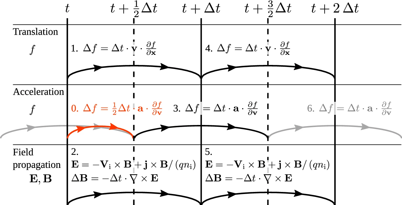
The splitting is performed using a leapfrog scheme:

$$\tilde{f}^{n+1} = S_A\left( \frac{\Delta t}{2}\right)\, S_T\left(\Delta t \right)\, S_A\left( \frac{\Delta t}{2}\right)\, \tilde{f}^n$$

$S_A$ can generally be described by an offset 3D rotation matrix (due to gyration around $\mathbf{B}$). As every offset rotation matrix can be decomposed into three shear matrices $S = S_x S_y S_z$, each performing an axis-parallel shear into one spatial dimension, the numerically efficient semi-Lagrangian acceleration update using the SLICE-3D approach is possible: before each shear transformation, the velocity space is rearranged into a single-cell column format parallel to the shear direction in memory, each of which requires only a 1D remapping with a high reconstruction order. This update method comes with a maximum rotation angle limit due to the shear decomposition of about 22∘ (WHY???), which imposes a further time step limit. For larger rotational angles per time step (caused by stronger magnetic fields), the acceleration can be subcycled.

$S_T$ can generally be described by a translation matrix with no rotation, and the same SLICE-3D approach lends itself to it in a similar vein as for velocity space. The main difference is the typical use of 3rd order reconstruction in order to keep the stencil width at two.

Field Propagation

The magnetic field is propagated using the algorithm by Londrillo and del Zanna (2004), which is a 2nd-order accurate (both in time and space) upwind constrained transport method. All reconstructions between volume-, face- and edge-averaged values follow Balsara+ (2009). The face-averaged values of $\mathbf{B}$ are propagated forward in time using the integral form of Faraday's law

$$\frac{\partial}{\partial t}\int_{\text{face}}\mathbf{B}\cdot d\mathbf{A} = -\oint_C \mathbf{E}\cdot d\mathbf{S},$$

where the integral on the LHS is taken over the cell face and the line integral is evaluated along the contour of that face. Once $\mathbf{E}$ has been computed based on Ohm's law, it is easy to propagate $\mathbf{B}$ using the discretized form of the above. When computing each component of $\mathbf{E}$ on an edge, the solver computes the candidate values on the four neighboring cells of the edge. In the supermagnetosonic case, when the plasma velocity exceeds the speed of the fast magnetosonic wave mode, the upwinded value from one of the cells is used. In the submagnetosonic case the value is computed as a weighted average of the electric field on the four cells and a diffusive flux is added to stabilize the scheme.

For the time integration a $2^{nd}$ order Runge–Kutta method is used. To propagate the field from $t$ to $t + \Delta t$ we need the $\rho_q$ and $\mathbf{V}_i$ values at both $t$ and $t + \Delta t/2$. With the leap-frog algorithm there are no real values for the distribution function at these times. A $1^{st}$ order accurate interpolation is used to compute the required values:

$$\tilde{f}(t) = \frac{1}{2}\big[ \tilde{f}^v(t) + \tilde{f}^r(t+\frac{1}{2}\Delta t) \big],$$ $$\tilde{f}(t+\frac{1}{2}\Delta t) = \frac{1}{2}\big[ \tilde{f}^v(t+\Delta t) + \tilde{f}^r(t+\frac{1}{2}\Delta t) \big].$$

The field solver also contributes to the dynamic computation of the timestep. With the simplest form of Ohm's law the fastest characteristic speed is the speed of the fast magnetosonic wave mode and we use that speed to compute the maximum timestep allowed by the field solver. For the field solver Courant numbers $\in [0.4, 0.5]$ is used, as higher values cause numerical instability of the scheme.

In Vlasiator the magnetic field has been split into a perturbed field updated during the simulations, and a static background field. The electric field is computed based on the total magnetic field and all changes to the magnetic field are only added to the perturbed part of the magnetic field. The background field must be curl-free and thus the Hall term can be computed based on the perturbed part only. This avoids numerical integration errors arising from strong background field gradients. In magnetospheric simulations the background field consists of the Earth's dipole, as well as a constant IMF in all cells. As can be seen in ldz_main.cpp, to handle the potential stiffness of the generalized Ohm's law, the subcycling technique (typically within 50 cycles) is applied for all terms on the RHS. Compared this to the MHD treatment in BATSRUS: BATSRUS solves the advection term $-\mathbf{u}\times\mathbf{B}$ and electron pressure gradient term $\nabla P_e/n$ are marched with explicit scheme, while the Hall term $\mathbf{j}\times\mathbf{B}$ is marched with implicit GMRES scheme (typically ~ 10 steps). This lies in the fact that the Hall term is mathematically stiff, while other terms are nonstiff. This makes me wondering if it is possible to use different treatment for different terms in Vlasiator as well.

When adapting to AMR, Vlasiator developers made the decision of first keeping the same field solver on the finest level only. This makes the efficient implementation easier, at the cost of memory usage.

Sparse Velocity Grid

A typical ion population is localized in velocity space, for example a Maxwellian distribution, and a large portion of velocity space is effectively empty. A key technique in saving memory is the sparse velocity grid storage. The velocity grid is divided into velocity blocks comprising 4x4x4 velocity cells. The sparse representation is done at this level: either a block exists with all of its 64 velocity cells, or it does not exist at all. In the sparse representation we define that a block has content if any of its 64 velocity cells has a density above a user-specified threshold value. A velocity block exists if it has content, or if it is a neighbor to a block with content in any of the six dimensions. In the velocity space all 26 nearest neighbors are included, while in ordinary space blocks within a distance of 2 in the 6 normal directions and a distance of 1 in nodal directions are included.

There are two sources of loss when propagating the distribution function:

1. fluxes that flow out of the velocity grid;

2. distributions that go below the storage threshold.

Usually the $1^{st}$ term dominates.^[2]

[1]	Eulerian and Lagrangian descriptions of field appear most notably in fluid mechanics.

[2]	This can be easily observed with a small velocity space, where the moments calculated from the distribution functions deviates from the analytical values.