FLEKS Python Visualization Toolkit
flekspy is a Python package for processing FLEKS data.
FLEKS data format
Field: *.out format or AMREX built-in format, whose directory name is assumed to end with “_amrex”
PIC particle: AMREX built-in format
Test particle: binary data format
Importing the package
import flekspy
Downloading demo data
If you don’t have FLEKS data to start with, you can download demo field data with the following:
from flekspy.util import download_testfile

url = "https://raw.githubusercontent.com/henry2004y/batsrus_data/master/batsrus_data.tar.gz"
download_testfile(url, "data")
Example test particle data can be downloaded as follows:
url = "https://raw.githubusercontent.com/henry2004y/batsrus_data/master/test_particles_PBEG.tar.gz"
download_testfile(url, "data")
Example PIC particle data can be downloaded as follows:
url = "https://raw.githubusercontent.com/henry2004y/batsrus_data/master/3d_particle.tar.gz"
download_testfile(url, "data")
Loading data
flekspy.load is the interface to read files of all formats. It returns a different object for different formats. IDL format data are processed into XArray data structures:
file = "data/1d__raw_2_t25.60000_n00000258.out"
ds = flekspy.load(file)
ds
<xarray.Dataset> Size: 31kB
Dimensions:  (x: 256)
Coordinates:
  * x        (x) float64 2kB -127.5 -126.5 -125.5 -124.5 ... 125.5 126.5 127.5
Data variables: (12/14)
    Rho      (x) float64 2kB 1.0 1.0 1.0 1.0 1.0 ... 0.125 0.125 0.125 0.125
    Mx       (x) float64 2kB 5.791e-14 1.309e-13 ... 1.92e-11 9.193e-12
    My       (x) float64 2kB 1.718e-13 5.386e-13 1.697e-12 ... 2.808e-11 1.2e-11
    Mz       (x) float64 2kB 0.0 0.0 0.0 0.0 0.0 0.0 ... 0.0 0.0 0.0 0.0 0.0 0.0
    Bx       (x) float64 2kB 0.2236 0.2236 0.2236 0.2236 ... 1.118 1.118 1.118
    By       (x) float64 2kB 1.23 1.23 1.23 1.23 ... -0.559 -0.559 -0.559 -0.559
    ...       ...
    E        (x) float64 2kB 1.781 1.781 1.781 1.781 ... 0.8813 0.8813 0.8813
    p        (x) float64 2kB 1.0 1.0 1.0 1.0 1.0 1.0 ... 0.1 0.1 0.1 0.1 0.1 0.1
    b1x      (x) float64 2kB 0.2236 0.2236 0.2236 0.2236 ... 1.118 1.118 1.118
    b1y      (x) float64 2kB 1.23 1.23 1.23 1.23 ... -0.559 -0.559 -0.559 -0.559
    b1z      (x) float64 2kB 0.0 0.0 0.0 0.0 0.0 0.0 ... 0.0 0.0 0.0 0.0 0.0 0.0
    absdivB  (x) float64 2kB 6.466e-13 1.994e-12 ... 2.394e-12 8.149e-12
Attributes: (12/20)
    filename:    /home/runner/work/flekspy/flekspy/docs/data/1d__raw_2_t25.60...
    isOuts:      False
    npict:       1
    nInstance:   1
    fileformat:  ascii
    unit:        normalized
    ...          ...
    para:        [3. 2. 0. 0.]
    dims:        ['x']
    variables:   ['x' 'Rho' 'Mx' 'My' 'Mz' 'Bx' 'By' 'Bz' 'Hyp' 'E' 'p' 'b1x'...
    strtime:     0000h00m25.600s
    param_name:  ['r' 'g' 'cuty' 'cutz']
registry: <unyt.unit_registry.UnitRegistry object at 0x7fe82f34a0b0>The coordinates can be accessed via
ds.coords
Coordinates:
* x (x) float64 2kB -127.5 -126.5 -125.5 -124.5 ... 125.5 126.5 127.5
The variables can be accessed via
ds.var
<bound method DatasetAggregations.var of <xarray.Dataset> Size: 31kB
Dimensions: (x: 256)
Coordinates:
* x (x) float64 2kB -127.5 -126.5 -125.5 -124.5 ... 125.5 126.5 127.5
Data variables: (12/14)
Rho (x) float64 2kB 1.0 1.0 1.0 1.0 1.0 ... 0.125 0.125 0.125 0.125
Mx (x) float64 2kB 5.791e-14 1.309e-13 ... 1.92e-11 9.193e-12
My (x) float64 2kB 1.718e-13 5.386e-13 1.697e-12 ... 2.808e-11 1.2e-11
Mz (x) float64 2kB 0.0 0.0 0.0 0.0 0.0 0.0 ... 0.0 0.0 0.0 0.0 0.0 0.0
Bx (x) float64 2kB 0.2236 0.2236 0.2236 0.2236 ... 1.118 1.118 1.118
By (x) float64 2kB 1.23 1.23 1.23 1.23 ... -0.559 -0.559 -0.559 -0.559
... ...
E (x) float64 2kB 1.781 1.781 1.781 1.781 ... 0.8813 0.8813 0.8813
p (x) float64 2kB 1.0 1.0 1.0 1.0 1.0 1.0 ... 0.1 0.1 0.1 0.1 0.1 0.1
b1x (x) float64 2kB 0.2236 0.2236 0.2236 0.2236 ... 1.118 1.118 1.118
b1y (x) float64 2kB 1.23 1.23 1.23 1.23 ... -0.559 -0.559 -0.559 -0.559
b1z (x) float64 2kB 0.0 0.0 0.0 0.0 0.0 0.0 ... 0.0 0.0 0.0 0.0 0.0 0.0
absdivB (x) float64 2kB 6.466e-13 1.994e-12 ... 2.394e-12 8.149e-12
Attributes: (12/20)
filename: /home/runner/work/flekspy/flekspy/docs/data/1d__raw_2_t25.60...
isOuts: False
npict: 1
nInstance: 1
fileformat: ascii
unit: normalized
... ...
para: [3. 2. 0. 0.]
dims: ['x']
variables: ['x' 'Rho' 'Mx' 'My' 'Mz' 'Bx' 'By' 'Bz' 'Hyp' 'E' 'p' 'b1x'...
strtime: 0000h00m25.600s
param_name: ['r' 'g' 'cuty' 'cutz']
registry: <unyt.unit_registry.UnitRegistry object at 0x7fe82f34a0b0>>
and individual variables can be accessed through keys or properties:
ds["p"]
ds.p
<xarray.DataArray 'p' (x: 256)> Size: 2kB
array([1.        , 1.        , 1.        , 1.        , 1.        ,
       1.        , 1.        , 1.        , 1.        , 1.        ,
       1.        , 1.        , 1.        , 0.99999999, 0.99999999,
       0.99999999, 0.99999998, 0.99999997, 0.99999996, 0.99999995,
       0.99999994, 0.99999992, 0.99999989, 0.99999986, 0.99999982,
       0.99999977, 0.99999971, 0.99999964, 0.99999955, 0.99999944,
       0.99999931, 0.99999915, 0.99999896, 0.99999873, 0.99999846,
       0.99999813, 0.99999775, 0.99999729, 0.99999676, 0.99999612,
       0.99999538, 0.9999945 , 0.99999348, 0.99999229, 0.99999089,
       0.99998927, 0.99998739, 0.9999852 , 0.99998266, 0.99997971,
       0.99997631, 0.99997238, 0.99996784, 0.99996262, 0.99995661,
       0.99994971, 0.9999418 , 0.99993277, 0.99992245, 0.99991061,
       0.99989688, 0.99988076, 0.99986169, 0.99983926, 0.99981363,
       0.99978593, 0.99975843, 0.99973409, 0.99971417, 0.99969689,
       0.99967628, 0.9996342 , 0.99948851, 0.99875656, 0.99520955,
       0.98644347, 0.97296833, 0.95605524, 0.93689582, 0.91642986,
       0.89531082, 0.87393959, 0.85255455, 0.83129714, 0.81025231,
       0.78947393, 0.76899764, 0.74884761, 0.72904066, 0.70958859,
       0.69049963, 0.67177964, 0.6534332 , 0.63546454, 0.6178779 ,
       0.60067737, 0.58386638, 0.56744599, 0.55141095, 0.5357435 ,
...
       0.51903728, 0.51937986, 0.51946056, 0.51934921, 0.51897835,
       0.51808309, 0.51597448, 0.50838603, 0.47777544, 0.37490815,
       0.18275943, 0.09437588, 0.08721111, 0.08711243, 0.08735865,
       0.08766624, 0.0878924 , 0.08798467, 0.08799348, 0.08798877,
       0.08797256, 0.08793813, 0.08786602, 0.08773117, 0.08758445,
       0.08751411, 0.08750803, 0.08751301, 0.08753202, 0.08757715,
       0.08762349, 0.0876353 , 0.08763337, 0.0876259 , 0.08760677,
       0.08758085, 0.08757283, 0.08757511, 0.0875862 , 0.0876146 ,
       0.08767738, 0.08777552, 0.08786197, 0.0878934 , 0.08789452,
       0.0878902 , 0.08787545, 0.08783555, 0.08774973, 0.08757955,
       0.08727059, 0.08688917, 0.08660118, 0.08652576, 0.08652704,
       0.08655168, 0.08662743, 0.08679863, 0.08714811, 0.08775512,
       0.08855411, 0.08946919, 0.09044863, 0.0914582 , 0.09247696,
       0.09349335, 0.09449866, 0.0954875 , 0.09645212, 0.0973789 ,
       0.09825058, 0.0990272 , 0.09964004, 0.09996659, 0.10003448,
       0.10004239, 0.10004135, 0.10003742, 0.10003136, 0.10002179,
       0.10001115, 0.10000324, 0.10000038, 0.1       , 0.09999996,
       0.09999996, 0.09999997, 0.09999999, 0.1       , 0.1       ,
       0.1       , 0.1       , 0.1       , 0.1       , 0.1       ,
       0.1       ])
Coordinates:
* x (x) float64 2kB -127.5 -126.5 -125.5 -124.5 ... 125.5 126.5 127.5Interpolating data
Variable interpolation is supported via XArray. For 1D data, simply provide the coordinate:
ds["Rho"].interp(x=100)
<xarray.DataArray 'Rho' ()> Size: 8B
array(0.12245273)
Coordinates:
x int64 8B 100For multidimensional interpolation, it can be easily extended as
file = "data/z=0_fluid_region0_0_t00001640_n00010142.out"
ds = flekspy.load(file)
ds["rhoS0"].interp(x=-28000.0, y =0.0)
<xarray.DataArray 'rhoS0' ()> Size: 8B
array(0.12202676)
Coordinates:
    x        float64 8B -2.8e+04
y float64 8B 0.0If you want to interpolate for all variables at a single location,
ds.interp(x=-28000.0, y =0.0)
<xarray.Dataset> Size: 240B
Dimensions:  ()
Coordinates:
    x        float64 8B -2.8e+04
    y        float64 8B 0.0
Data variables: (12/28)
    rhoS0    float64 8B 0.122
    rhoS1    float64 8B 12.28
    Bx       float64 8B 0.2617
    By       float64 8B 0.1596
    Bz       float64 8B 20.24
    Ex       float64 8B 411.3
    ...       ...
    pXXS1    float64 8B 0.4068
    pYYS1    float64 8B 0.3315
    pZZS1    float64 8B 0.08105
    pXYS1    float64 8B -0.0111
    pXZS1    float64 8B -0.004809
    pYZS1    float64 8B 0.008121
Attributes: (12/23)
    filename:    /home/runner/work/flekspy/flekspy/docs/data/z=0_fluid_region...
    isOuts:      False
    npict:       1
    nInstance:   1
    fileformat:  binary
    end_char:    <
    ...          ...
    para:        [ 9.99999978e-03 -2.50000000e-01  1.00000000e+00  2.50000000...
    dims:        ['x', 'y']
    variables:   ['x' 'y' 'rhoS0' 'rhoS1' 'Bx' 'By' 'Bz' 'Ex' 'Ey' 'Ez' 'uxS0...
    strtime:     0000h16m40.021s
    param_name:  ['mS0' 'qS0' 'mS1' 'qS1' 'cLight' 'rPlanet' 'cutz']
registry: <unyt.unit_registry.UnitRegistry object at 0x7fe82f32e1a0>Visualizing fields
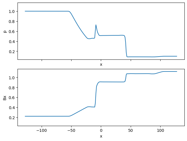
Thanks to XArray’s Matplotlib wrapper, all Matplotlib’s plotting functionalities are directly supported.
import matplotlib.pyplot as plt

file = "data/1d__raw_2_t25.60000_n00000258.out"
ds = flekspy.load(file)

fig, axs = plt.subplots(2, 1, constrained_layout=True, sharex=True, sharey=True)
ds.p.plot(ax=axs[0])
ds.Bx.plot(ax=axs[1])
plt.show()
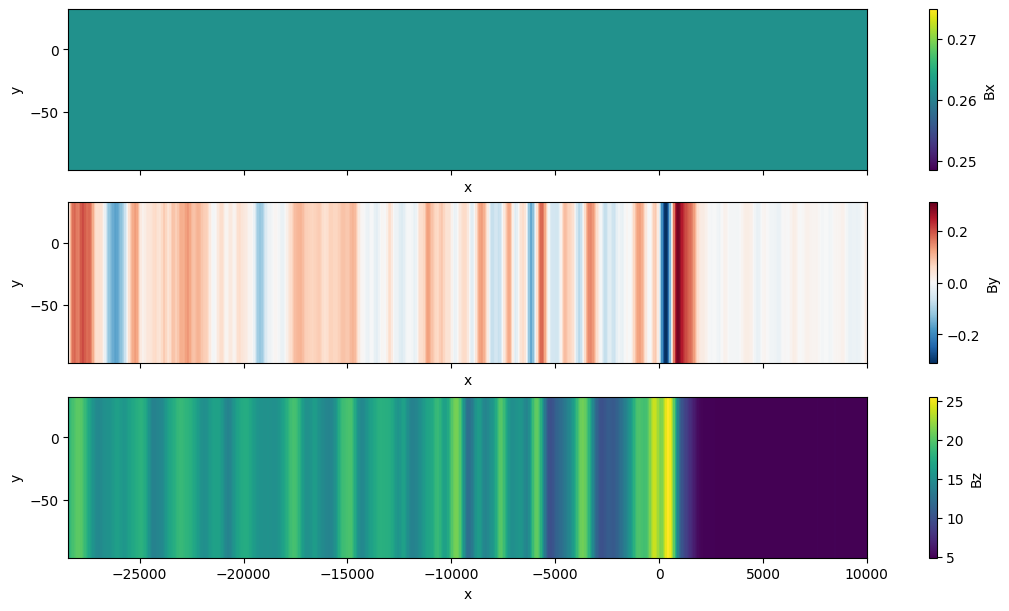
By default, XArray’s 2D plotting functions map the first dimension to the vertical y-axis and the second dimension to the horizontal x-axis. To overwrite this default behavior, we can explicitly set the x and y arguments:
file = "data/z=0_fluid_region0_0_t00001640_n00010142.out"
ds = flekspy.load(file)
fig, axs = plt.subplots(3, 1, figsize=(10, 6), constrained_layout=True, sharex=True, sharey=True)
ds.Bx.plot.pcolormesh(ax=axs[0], x="x", y="y")
ds.By.plot.pcolormesh(ax=axs[1], x="x", y="y")
ds.Bz.plot.pcolormesh(ax=axs[2], x="x", y="y")
plt.show()
Native AMReX format can be read using YT:
ds = flekspy.load("data/3d*amrex")
yt : [INFO ] 2025-09-10 16:40:13,617 Parameters: current_time = 2.066624095642792
yt : [INFO ] 2025-09-10 16:40:13,617 Parameters: domain_dimensions = [64 40 1]
yt : [INFO ] 2025-09-10 16:40:13,618 Parameters: domain_left_edge = [-0.016 -0.01 0. ]
yt : [INFO ] 2025-09-10 16:40:13,619 Parameters: domain_right_edge = [0.016 0.01 1. ]
We can take a slice at a given location, which works both for IDL and AMReX data:
dc = ds.get_slice("z", 0.5)
dc
variables : ['particle_cpu', 'particle_id', 'particle_position_x', 'particle_position_y', 'particle_supid', 'particle_velocity_x', 'particle_velocity_y', 'particle_velocity_z', 'particle_weight', 'Bx', 'By', 'Bz', 'Ex', 'Ey', 'Ez']
data range: [[unyt_quantity(-0.016, 'code_length'), unyt_quantity(0.016, 'code_length')], [unyt_quantity(-0.01, 'code_length'), unyt_quantity(0.01, 'code_length')], [0, 0]]
dimension : (256423,)
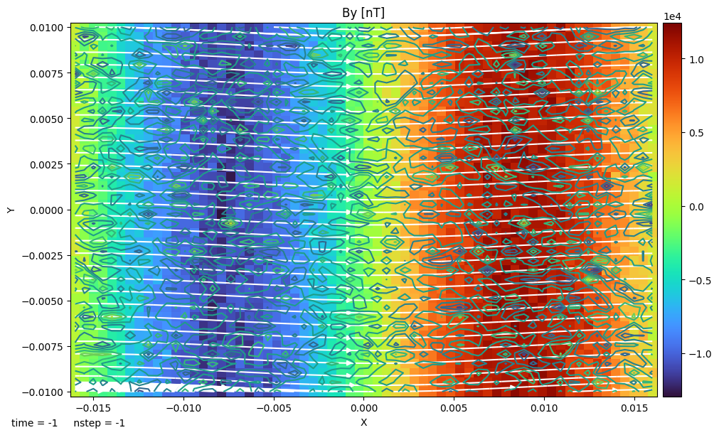
and plot the selected variables on the slice with colored contours, streamlines, and contour lines:
f, axes = dc.plot("By", pcolor=True)
dc.add_stream(axes[0], "Bx", "By", color="w")
dc.add_contour(axes[0], "Bx")
[2025-09-10 16:40:13,921] [flekspy.util.data_container] [INFO] Plots at z = 0.5 code_length
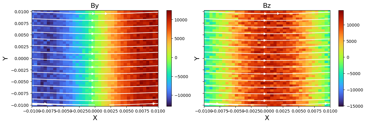
Users can also obtain the data of a 2D plane, and visualize it with matplotlib. A complete example is given below:
import matplotlib.pyplot as plt
import numpy as np

ds = flekspy.load("data/3*amrex")
dc = ds.get_slice("z", 0.5)

f, axes = plt.subplots(
    1, 2, figsize=(12, 4), constrained_layout=True, sharex=True, sharey=True
)

fields = ["By", "Bz"]
for ivar in range(2):
    v = dc.evaluate_expression(fields[ivar])
    vmin = v.min().v
    vmax = v.max().v
    ax = axes[ivar]
    ax.set_title(fields[ivar], fontsize=16)
    ax.set_ylabel("Y", fontsize=16)
    ax.set_xlabel("X", fontsize=16)
    c = ax.pcolormesh(dc.x.value, dc.y.value, np.array(v.T), cmap="turbo")
    cb = f.colorbar(c, ax=ax, pad=0.01)

    ax.set_xlim(np.min(dc.x.value), np.max(dc.x.value))
    ax.set_xlim(np.min(dc.y.value), np.max(dc.y.value))
    dc.add_stream(ax, "Bx", "By", density=0.5, color="w")

plt.show()
yt : [INFO ] 2025-09-10 16:40:14,525 Parameters: current_time = 2.066624095642792
yt : [INFO ] 2025-09-10 16:40:14,525 Parameters: domain_dimensions = [64 40 1]
yt : [INFO ] 2025-09-10 16:40:14,526 Parameters: domain_left_edge = [-0.016 -0.01 0. ]
yt : [INFO ] 2025-09-10 16:40:14,526 Parameters: domain_right_edge = [0.016 0.01 1. ]
Visualizing phase space distributions
from flekspy.util import unit_one

data_file = "data/3d_*amrex"
ds = flekspy.load(data_file)

# Add a user defined field. See yt document for more information about derived field.
ds.add_field(
    ds.pvar("unit_one"),
    function=unit_one,
    sampling_type="particle",
    units="dimensionless",
)

x_field = "p_uy"
y_field = "p_uz"
# z_field = "unit_one"
z_field = "p_w"
xleft = [-0.016, -0.01, 0.0]
xright = [0.016, 0.01, 1.0]

zmin, zmax = 1e-5, 2e-3

## Select and plot the particles inside a box defined by xleft and xright
region = ds.box(xleft, xright)
pp = ds.plot_phase(
    x_field,
    y_field,
    z_field,
    region=region,
    unit_type="si",
    x_bins=100,
    y_bins=32,
    domain_size=(xleft[0], xright[0], xleft[1], xright[1]),
)

pp.set_cmap(pp.fields[0], "turbo")
pp.set_font(
    {
        "size": 34,
        "family": "DejaVu Sans",
    }
)

pp.set_zlim(pp.fields[0], zmin=zmin, zmax=zmax)

pp.set_xlabel(r"$V_y$")
pp.set_ylabel(r"$V_z$")
pp.set_colorbar_label(pp.fields[0], "weight")
str_title = (
    rf"x = [{xleft[0]:.1e}, {xright[0]:.1e}], y = [{xleft[1]:.1e}, {xright[1]:.1e}]"
)
pp.set_title(pp.fields[0], str_title)
pp.set_log(pp.fields[0], True)
pp.show()
# pp.save("test")
# pp.plots[("particles", z_field)].axes.xaxis.set_major_locator(
# ticker.MaxNLocator(4))
# pp.plots[("particles", z_field)].axes.yaxis.set_major_locator(
# ticker.MaxNLocator(4))
yt : [INFO ] 2025-09-10 16:40:15,268 Parameters: current_time = 2.066624095642792
yt : [INFO ] 2025-09-10 16:40:15,269 Parameters: domain_dimensions = [64 40 1]
yt : [INFO ] 2025-09-10 16:40:15,269 Parameters: domain_left_edge = [-0.016 -0.01 0. ]
yt : [INFO ] 2025-09-10 16:40:15,270 Parameters: domain_right_edge = [0.016 0.01 1. ]

Plot the location of particles that are inside a sphere
center = [0, 0, 0]
radius = 1
# Object sphere is defined in yt/data_objects/selection_objects/spheroids.py
sp = ds.sphere(center, radius)
pp = ds.plot_particles(
    "p_x", "p_y", "p_w", region=sp, unit_type="si", x_bins=64, y_bins=64
)
pp.show()
# pp.save("test")
yt : [INFO ] 2025-09-10 16:40:15,855 xlim = -0.016000 0.016000
yt : [INFO ] 2025-09-10 16:40:15,856 ylim = -0.010000 0.010000
yt : [INFO ] 2025-09-10 16:40:15,857 xlim = -0.016000 0.016000
yt : [INFO ] 2025-09-10 16:40:15,858 ylim = -0.010000 0.010000
yt : [INFO ] 2025-09-10 16:40:15,861 Splatting (('particles', 'p_w')) onto a 800 by 800 mesh using method 'ngp'

Plot the velocity space of particles that are inside a sphere
pp = ds.plot_phase(
    "p_uy", "p_uz", "p_w", region=sp, unit_type="si", x_bins=64, y_bins=64
)

pp.set_cmap(pp.fields[0], "turbo")

pp.set_font(

    {

        "size": 34,

        "family": "DejaVu Sans",

    }
)

pp.show()

Plot the location of particles that are inside a disk
center = [0, 0, 0]
normal = [0, 0, 1]  # normal direction of the disk
radius = 0.5
height = 1.0
# Object sphere is defined in yt/data_objects/selection_objects/disk.py
disk = ds.disk(center, normal, radius, height)
pp = ds.plot_particles(
    "p_x", "p_y", "p_w", region=disk, unit_type="si", x_bins=64, y_bins=64
)
pp.show()
yt : [INFO ] 2025-09-10 16:40:17,041 xlim = -0.016000 0.016000
yt : [INFO ] 2025-09-10 16:40:17,041 ylim = -0.010000 0.010000
yt : [INFO ] 2025-09-10 16:40:17,043 xlim = -0.016000 0.016000
yt : [INFO ] 2025-09-10 16:40:17,044 ylim = -0.010000 0.010000
yt : [INFO ] 2025-09-10 16:40:17,044 Splatting (('particles', 'p_w')) onto a 800 by 800 mesh using method 'ngp'
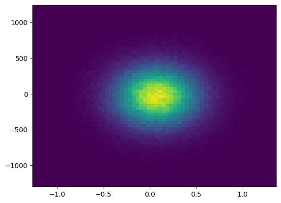
Plot the velocity space of particles that are inside a disk
pp = ds.plot_phase(
    "p_uy", "p_uz", "p_w", region=disk, unit_type="si", x_bins=64, y_bins=64
)

pp.show()

Get the 2D array from the phase plot and reconstruct from scratch:
for var_name in pp.profile.field_data:
    val = pp.profile.field_data[var_name]

x = pp.profile.x
y = pp.profile.y

plt.pcolormesh(x, y, val)
plt.show()
Plotting Test Particle Trajectories
Loading particle data
from flekspy import FLEKSTP

tp = FLEKSTP("data/test_particles_PBEG", iSpecies=1)
Obtaining particle IDs
Test particle IDs consists of a CPU index and a particle index attached to the CPU.
tp.getIDs()
[(0, 3), (0, 4)]
Reading particle trajectory
tp[0].collect()
| time | x | y | z | vx | vy | vz | bx | by | bz | ex | ey | ez | dbxdx | dbxdy | dbxdz | dbydx | dbydy | dbydz | dbzdx | dbzdy | dbzdz |
|---|---|---|---|---|---|---|---|---|---|---|---|---|---|---|---|---|---|---|---|---|---|
| f32 | f32 | f32 | f32 | f32 | f32 | f32 | f32 | f32 | f32 | f32 | f32 | f32 | f32 | f32 | f32 | f32 | f32 | f32 | f32 | f32 | f32 |
| 0.0 | 0.000128 | -0.000795 | 0.0 | 0.000042 | 0.000067 | 0.000016 | 224199.65625 | 281.65274 | 11182.642578 | -0.447306 | 3.064687 | 8.890797 | 0.0 | 0.0 | 0.0 | 2.1949e6 | 0.0 | 0.0 | -107828.21875 | 0.0 | 0.0 |
| 0.286543 | 0.000134 | -0.000786 | 0.000002 | 0.000042 | 0.000068 | 0.000014 | 224414.28125 | 207.771286 | 11134.431641 | -1.991942 | 3.305334 | 8.97459 | -225897.34375 | 123607.867188 | 0.0 | 1.993212e6 | 110127.578125 | 0.0 | -52048.246094 | 458591.0 | 0.0 |
| 0.573086 | 0.000146 | -0.000766 | 0.000002 | 0.000042 | 0.000069 | 0.000012 | 224547.4375 | 171.823151 | 11111.666016 | -1.018998 | 2.346379 | 8.844476 | -159384.8125 | 358307.84375 | 0.0 | 2.0199e6 | 25620.753906 | 0.0 | 68019.898438 | 1.3220e6 | 0.0 |
| 0.864857 | 0.000159 | -0.000745 | 0.000002 | 0.000042 | 0.000071 | 0.000011 | 224356.78125 | 25.654217 | 11075.149414 | 1.378713 | 3.30056 | 9.281602 | 385832.53125 | 685539.1875 | 0.0 | 2.0586e6 | -450143.34375 | 0.0 | 668866.25 | 693783.875 | 0.0 |
| 1.157084 | 0.000171 | -0.000724 | 0.000001 | 0.000043 | 0.000072 | 0.000009 | 224224.421875 | -133.657379 | 10893.328125 | 0.683855 | 2.13601 | 9.826899 | 822001.0 | 1.3780e6 | 0.0 | 1.7280e6 | -886848.8125 | 0.0 | 1.0217e6 | -653294.8125 | 0.0 |
Getting initial location
x = tp.read_initial_condition(tp.getIDs()[0])
print("time, X, Y, Z, Vx, Vy, Vz")
print(
    f"{x[0]:.2e}, {x[1]:.2e}, {x[2]:.2e}, {x[3]:.2e}, {x[4]:.2e}, {x[5]:.2e}, {x[6]:.2e}"
)
time, X, Y, Z, Vx, Vy, Vz
0.00e+00, 1.28e-04, -7.95e-04, 0.00e+00, 4.21e-05, 6.65e-05, 1.55e-05
Interpolate particles trajectory at selected times
from flekspy.tp import interpolate_at_times

interpolate_at_times(tp[0], [1.0])
| time | x | y | z | vx | vy | vz | bx | by | bz | ex | ey | ez | dbxdx | dbxdy | dbxdz | dbydx | dbydy | dbydz | dbzdx | dbzdy | dbzdz |
|---|---|---|---|---|---|---|---|---|---|---|---|---|---|---|---|---|---|---|---|---|---|
| f32 | f32 | f32 | f32 | f32 | f32 | f32 | f32 | f32 | f32 | f32 | f32 | f32 | f32 | f32 | f32 | f32 | f32 | f32 | f32 | f32 | f32 |
| 1.0 | 0.000165 | -0.000736 | 0.000001 | 0.000042 | 0.000071 | 0.00001 | 224295.5625 | -48.021412 | 10991.063477 | 1.057367 | 2.761999 | 9.533781 | 587544.0625 | 1.0058e6 | 0.0 | 1.90571e6 | -652103.1875 | 0.0 | 832021.6875 | 70810.625 | 0.0 |
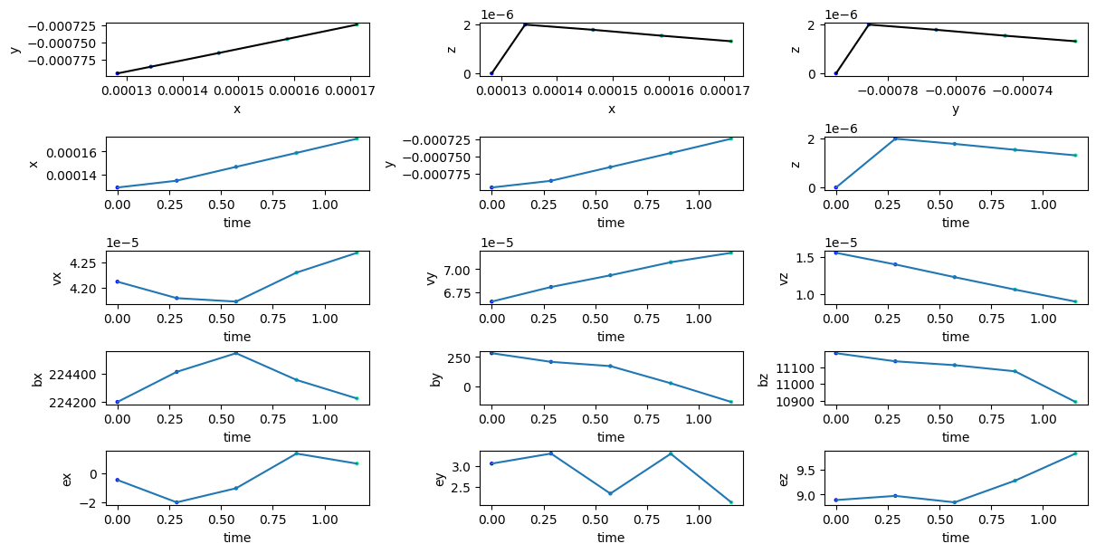
Plotting trajectory
tp.plot_trajectory(tp.getIDs()[0])
plt.show()
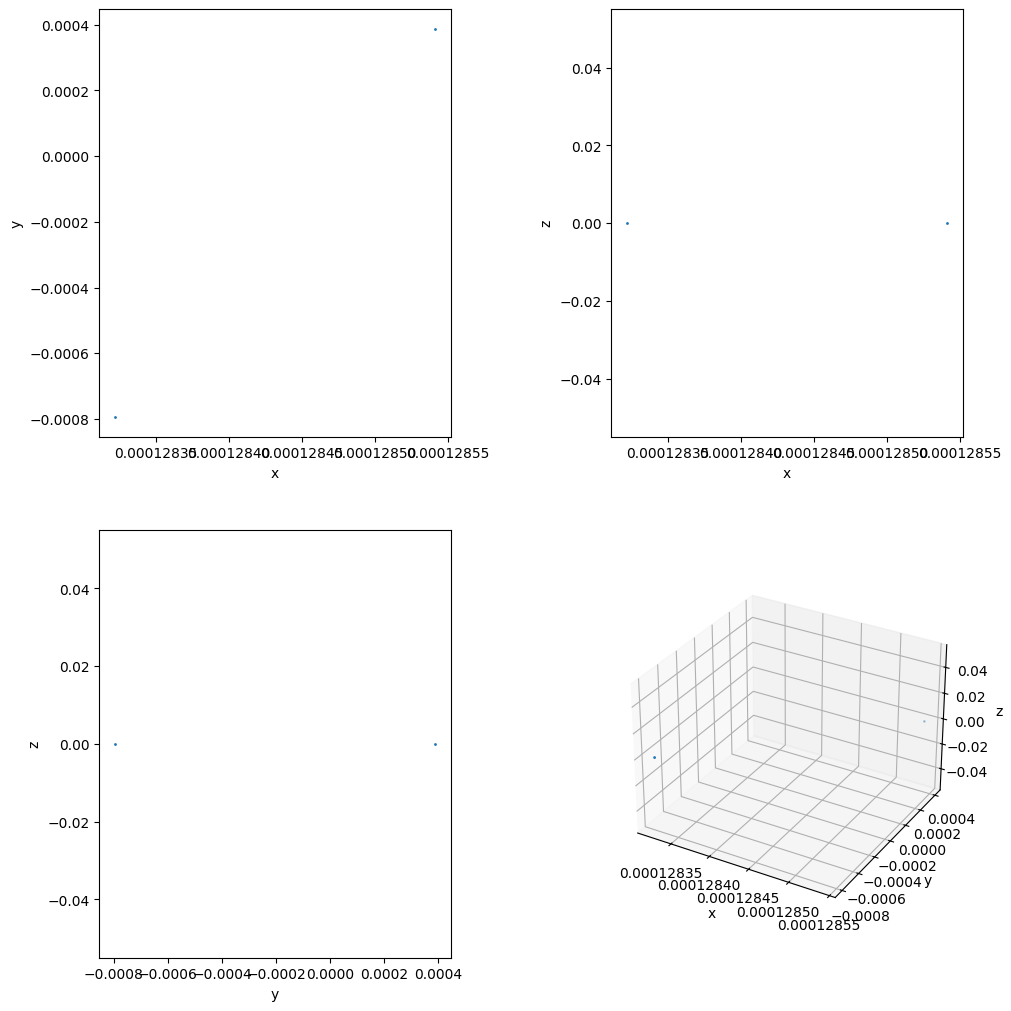
Reading and visualizing all particle’s location at a given snapshot
ids, pData = tp.read_particles_at_time(0.0, doSave=False)
tp.plot_location(pData)
plt.show()
Selecting particles starting in a region
from flekspy.tp import Indices

def f_select(tp, pid):
    pData = tp.read_initial_condition(pid)
    inRegion = pData[Indices.X] > 0 and pData[Indices.Y] > 0
    return inRegion


pSelected = tp.select_particles(f_select)
Saving trajectories to CSV
tp.save_trajectory_to_csv(tp.getIDs()[0])
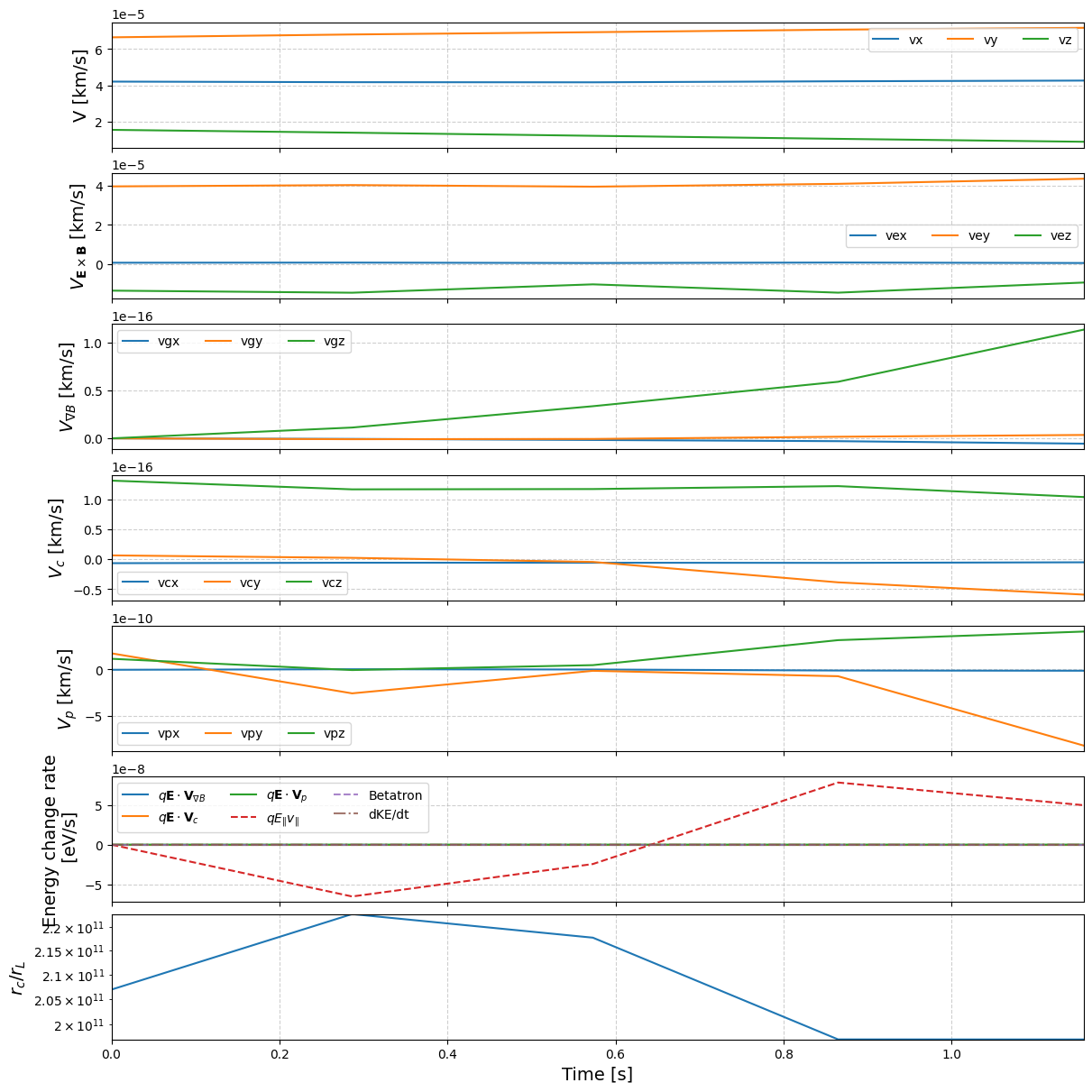
Calculating drifts
With the $\mathbf{E}, \mathbf{B}$, and $\nabla \mathbf{B}$ saved along the trajectory, we can compute various drifts:
Convection drift velocity:
tp.get_ExB_drift(pid)Curvature drift velocity:
tp.get_curvature_drift(pid)Gradient drift velocity:
tp.get_gradient_drift(pid)Polarization drift velocity:
tp.get_polarization_drift(pid)
The first adiabatic assumption can be checked by comparing the ratio between the curvature length and the gyroradius $r_c / r_L$ via get_adiabaticity_parameter. If $r_c / r_L \gg 1$, then the gyromotion can be savely ignored.
The Betatron acceleration $\mu \partial B/\partial t$ can be indirectly computed with the knowledge of total derivative $\mathrm{d}B/\mathrm{d}t$ and $\mathbf{v}\nabla B$ along the trajectory:
pid = tp.getIDs()[0]
pt = tp[pid]
mu = tp.get_first_adiabatic_invariant(pt)
pt = tp.get_betatron_acceleration(pt, mu)
To analyze a specific drift:
tp.analyze_drift(pid, "gradient")
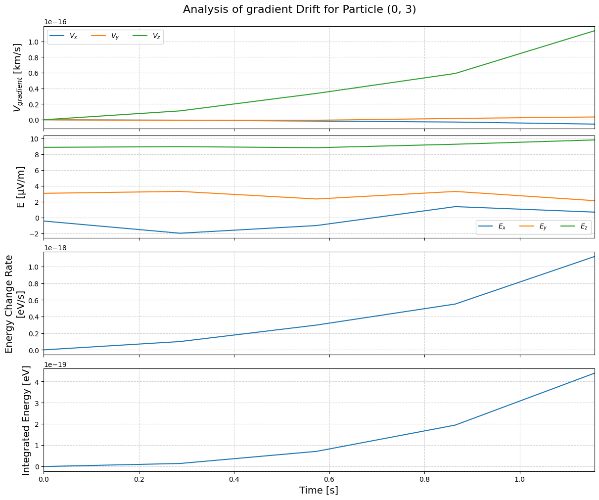
By combining all these together, we come up with time series of various terms:
tp.analyze_drifts(pid)
We can the track the energy change from drift and EM field variations:
from flekspy.tp import plot_integrated_energy

df = tp.integrate_drift_accelerations(tp.getIDs()[0])
plot_integrated_energy(df)
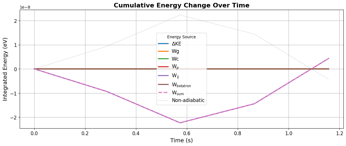
Alternatively, the energy change can be decomposed into three terms: the parallel acceleration, Betatron acceleration, and the Fermi acceleration:
df = tp.get_energy_change_guiding_center(tp.getIDs()[0])

df
| time | dW_parallel | dW_betatron | dW_fermi | dW_total |
|---|---|---|---|---|
| f32 | f32 | f32 | f32 | f32 |
| 0.0 | -1.2793e-15 | 7.9045e-14 | 1.1878e-18 | 7.7767e-14 |
| 0.286543 | -6.5532e-8 | 6.6485e-14 | 1.0648e-18 | -6.5532e-8 |
| 0.573086 | -2.4509e-8 | -1.0753e-14 | 1.0303e-18 | -2.4509e-8 |
| 0.864857 | 7.8494e-8 | -6.7355e-14 | 9.9597e-19 | 7.8494e-8 |
| 1.157084 | 4.9847e-8 | -5.8379e-14 | 8.8976e-19 | 4.9847e-8 |