Analyzing AMReX Outputs From FLEKS
In this demo, we show how to analyze native AMReX field and particle outputs. Example data can be downloaded as follows:
import flekspy
from flekspy.util import download_testfile

url = "https://raw.githubusercontent.com/henry2004y/batsrus_data/master/fleks_particle_small.tar.gz"
download_testfile(url, "data")
Inheriting from the IDL procedures, we can pass strings to limit the plotting range (experimental, may be changed in the future):
ds = flekspy.load("data/fleks_particle_small/3d*amrex")
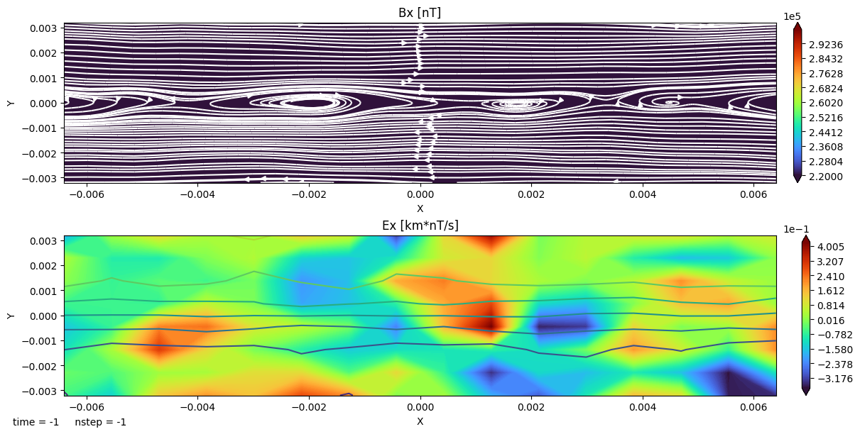
dc = ds.get_slice("z", 0.001)
f, axes = dc.plot("Bx>(2.2e5)<(3e5) Ex", figsize=(12, 6))
dc.add_stream(axes[0], "Bx", "By", color="w")
dc.add_contour(axes[1], "Bx", color="k")
yt : [INFO ] 2025-09-10 16:40:05,671 Parameters: current_time = 40.0
yt : [INFO ] 2025-09-10 16:40:05,672 Parameters: domain_dimensions = [16 8 6]
yt : [INFO ] 2025-09-10 16:40:05,672 Parameters: domain_left_edge = [-0.0064 -0.0032 -0.0024]
yt : [INFO ] 2025-09-10 16:40:05,673 Parameters: domain_right_edge = [0.0064 0.0032 0.0024]
[2025-09-10 16:40:06,031] [flekspy.util.data_container] [INFO] Plots at z = 0.001 code_length
/home/runner/work/flekspy/flekspy/src/flekspy/util/data_container.py:505: UserWarning: The following kwargs were not used by contour: 'color'
  ax.contour(self.x, self.y, v.T, *args, **kwargs)
Velocity Space Distributions
from flekspy.util import unit_one

filename = "data/fleks_particle_small/cut_*amrex"
ds = flekspy.load(filename)

# Add a user defined field. See yt document for more information about derived field.
ds.add_field(
    ds.pvar("unit_one"), function=unit_one, sampling_type="particle", units="code_mass"
)

x_field = "p_uy"
y_field = "p_uz"
z_field = "unit_one"
# z_field = "p_w"
xleft = [-0.001, -0.001, -0.001]
xright = [0.001, 0.001, 0.001]

### Select and plot the particles inside a box defined by xleft and xright
region = ds.box(xleft, xright)
pp = ds.plot_phase(
    x_field,
    y_field,
    z_field,
    region=region,
    unit_type="si",
    x_bins=64,
    y_bins=64,
    domain_size=(-0.0002, 0.0002, -0.0002, 0.0002),
)

pp.set_cmap(pp.fields[0], "turbo")

# plot.set_zlim(plot.fields[0], zmin, zmax)
pp.set_xlabel(r"$V_y$")
pp.set_ylabel(r"$V_z$")
# pp.set_colorbar_label(pp.fields[0], "pw")
pp.set_title(pp.fields[0], "Number density")
pp.set_font(
    {
        "size": 34,
        "family": "DejaVu Sans",
    }
)
pp.set_log(pp.fields[0], False)
pp.show()
yt : [INFO ] 2025-09-10 16:40:06,988 Parameters: current_time = 40.0
yt : [INFO ] 2025-09-10 16:40:06,988 Parameters: domain_dimensions = [16 8 6]
yt : [INFO ] 2025-09-10 16:40:06,989 Parameters: domain_left_edge = [-0.0064 -0.0032 -0.0024]
yt : [INFO ] 2025-09-10 16:40:06,989 Parameters: domain_right_edge = [0.0064 0.0032 0.0024]

If you need the direct phase space distributions together with the axis,
x, y, w = ds.get_phase(
    x_field,
    y_field,
    z_field,
    region=region,
    x_bins=64,
    y_bins=64,
    domain_size=(-0.0002, 0.0002, -0.0002, 0.0002),
)
To check the newly added field,
ad = ds.all_data()
ad[("particles", "unit_one")]
unyt_array([1., 1., 1., ..., 1., 1., 1.], shape=(3512,), units='code_mass')
Plot the location of particles that are inside a sphere
center = [0, 0, 0]
radius = 0.001
z_field = "unit_one"
# Object sphere is defined in yt/data_objects/selection_objects/spheroids.py
sp = ds.sphere(center, radius)
pp = ds.plot_particles(
    "p_x", "p_y", z_field, region=sp, unit_type="planet", x_bins=64, y_bins=64
)
pp.show()
yt : [INFO ] 2025-09-10 16:40:07,678 xlim = -0.006400 0.006400
yt : [INFO ] 2025-09-10 16:40:07,679 ylim = -0.003200 0.003200
yt : [INFO ] 2025-09-10 16:40:07,681 xlim = -0.006400 0.006400
yt : [INFO ] 2025-09-10 16:40:07,681 ylim = -0.003200 0.003200
yt : [INFO ] 2025-09-10 16:40:07,683 Splatting (('particles', 'unit_one')) onto a 800 by 800 mesh using method 'ngp'

Plot the phase space of particles that are inside a sphere
pp = ds.plot_phase(
    "p_uy", "p_uz", z_field, region=sp, unit_type="planet", x_bins=64, y_bins=64
)
pp.show()

Plot the location of particles that are inside a disk
center = [0, 0, 0]
normal = [1, 1, 0]
radius = 0.0005
height = 0.0004
z_field = "unit_one"
# Object sphere is defined in yt/data_objects/selection_objects/disk.py
disk = ds.disk(center, normal, radius, height)
pp = ds.plot_particles(
    "p_x", "p_y", z_field, region=disk, unit_type="planet", x_bins=64, y_bins=64
)
pp.show()
yt : [INFO ] 2025-09-10 16:40:08,357 xlim = -0.006400 0.006400
yt : [INFO ] 2025-09-10 16:40:08,358 ylim = -0.003200 0.003200
yt : [INFO ] 2025-09-10 16:40:08,360 xlim = -0.006400 0.006400
yt : [INFO ] 2025-09-10 16:40:08,360 ylim = -0.003200 0.003200
yt : [INFO ] 2025-09-10 16:40:08,361 Splatting (('particles', 'unit_one')) onto a 800 by 800 mesh using method 'ngp'

Plot the phase space of particles that are inside a disk
pp = ds.plot_phase(
    "p_uy", "p_uz", z_field, region=disk, unit_type="planet", x_bins=64, y_bins=64
)
pp.show()

Transform the velocity coordinates and visualize the phase space distribution
WIP
import flekspy, yt

l = [1, 0, 0]
m = [0, 1, 0]
n = [0, 0, 1]


def _vel_l(field, data):
    res = (
        l[0] * data[("particles", "p_ux")]
        + l[1] * data[("particles", "p_uy")]
        + l[2] * data[("particles", "p_uz")]
    )
    return res


def _vel_m(field, data):
    res = (
        m[0] * data[("particles", "p_ux")]
        + m[1] * data[("particles", "p_uy")]
        + m[2] * data[("particles", "p_uz")]
    )
    return res


def _vel_n(field, data):
    res = (
        n[0] * data[("particles", "p_ux")]
        + n[1] * data[("particles", "p_uy")]
        + n[2] * data[("particles", "p_uz")]
    )
    return res


filename = "data/fleks_particle_small/cut_*amrex"
ds = flekspy.load(filename)

# Add a user defined field. See yt document for more information about derived field.
vl_name = ds.pvar("vel_l")
vm_name = ds.pvar("vel_m")
vn_name = ds.pvar("vel_n")
ds.add_field(vl_name, units="code_velocity", function=_vel_l, sampling_type="particle")
ds.add_field(vm_name, units="code_velocity", function=_vel_m, sampling_type="particle")
ds.add_field(vn_name, units="code_velocity", function=_vel_n, sampling_type="particle")

######## Plot the location of particles that are inside a sphere ###########
center = [0, 0, 0]
radius = 0.001
# Object sphere is defined in yt/data_objects/selection_objects/spheroids.py
sp = ds.sphere(center, radius)

x_field = vl_name
y_field = vm_name
z_field = ds.pvar("p_w")

logs = {x_field: False, y_field: False}
profile = yt.create_profile(
    data_source=sp,
    bin_fields=[x_field, y_field],
    fields=z_field,
    n_bins=[64, 64],
    weight_field=None,
    logs=logs,
)

pp = yt.PhasePlot.from_profile(profile)

pp.set_unit(x_field, "km/s")
pp.set_unit(y_field, "km/s")
pp.set_unit(z_field, "amu")

pp.set_cmap(pp.fields[0], "turbo")
# pp.set_zlim(pp.fields[0], zmin, zmax)
pp.set_xlabel(r"$V_l$")
pp.set_ylabel(r"$V_m$")
pp.set_colorbar_label(pp.fields[0], "colorbar_label")
pp.set_title(pp.fields[0], "Density")
pp.set_font(
    {
        "size": 34,
        "family": "DejaVu Sans",
    }
)
pp.set_log(pp.fields[0], False)
pp.show()
yt : [INFO ] 2025-09-10 16:40:09,157 Parameters: current_time = 40.0
yt : [INFO ] 2025-09-10 16:40:09,157 Parameters: domain_dimensions = [16 8 6]
yt : [INFO ] 2025-09-10 16:40:09,158 Parameters: domain_left_edge = [-0.0064 -0.0032 -0.0024]
yt : [INFO ] 2025-09-10 16:40:09,158 Parameters: domain_right_edge = [0.0064 0.0032 0.0024]
