Cross-Wavelet Transform

Before we talk about cross-wavelet transform (CWT)¹, we need to understand wavelet transform (WT). Before we learn wavelet transform, we’d better have a good understanding of Fourier transform. Take a look at wavelet transform before moving on.

The cross-wavelet transform (CWT) method is a technique that characterizes the interaction between the wavelet transform (WT) of two individual time-series.²

The CWT method allows us to measure

• the degree of synchronization phenomenon between different components
• the evolution over time of the times-series data set.

Similarity/differences between two time-series can be identified. If these behavioral states have different temporal evolution, the CWT method helps quantifying how different they are, and what the time lag between the two different behavioral states is. In short, this method is able to yield information on the spatio-temporal organization between two time-series.

Synchronization

If you calculate the linear correlation between two time-series, you will get one value for the whole data; if you calculate the “local” linear correlation, you will get a 1D line values; if you perform CWT, you will get a 2D spectrum, i.e. the correlation at a given frequency at a given time.

So far, the Hilbert transform seems to be a relevant method to detect the phase synchronization between two time-series providing that the components of the time-series possess the same frequencies. However, this method cannot be directly applied to the analysis of the phase synchronization between two plurifrequential components of a time-series. A plurifrequential time-series is composed of a time-series with multiple frequencies occurring in the same time as it is commonly the case in living systems. The CWT method would be able to deal with such plurifrequential time-series and is conjointly able to detect the phase synchronization of such time-series.

Relative Phase

CWT can measure the ordering of the interaction among components, or in a continuous manner, lag.

Requirements

• Same duration for the two time-series
• Similar sampling rate (downsampling may be useful if one of the time-series has a higher sampling rate than the other)

Example

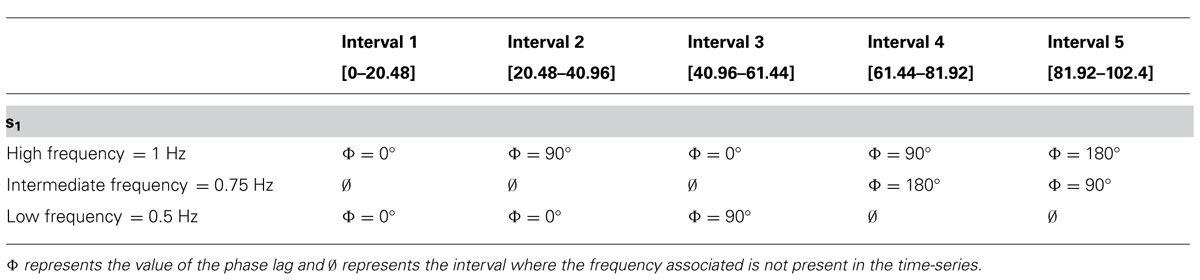
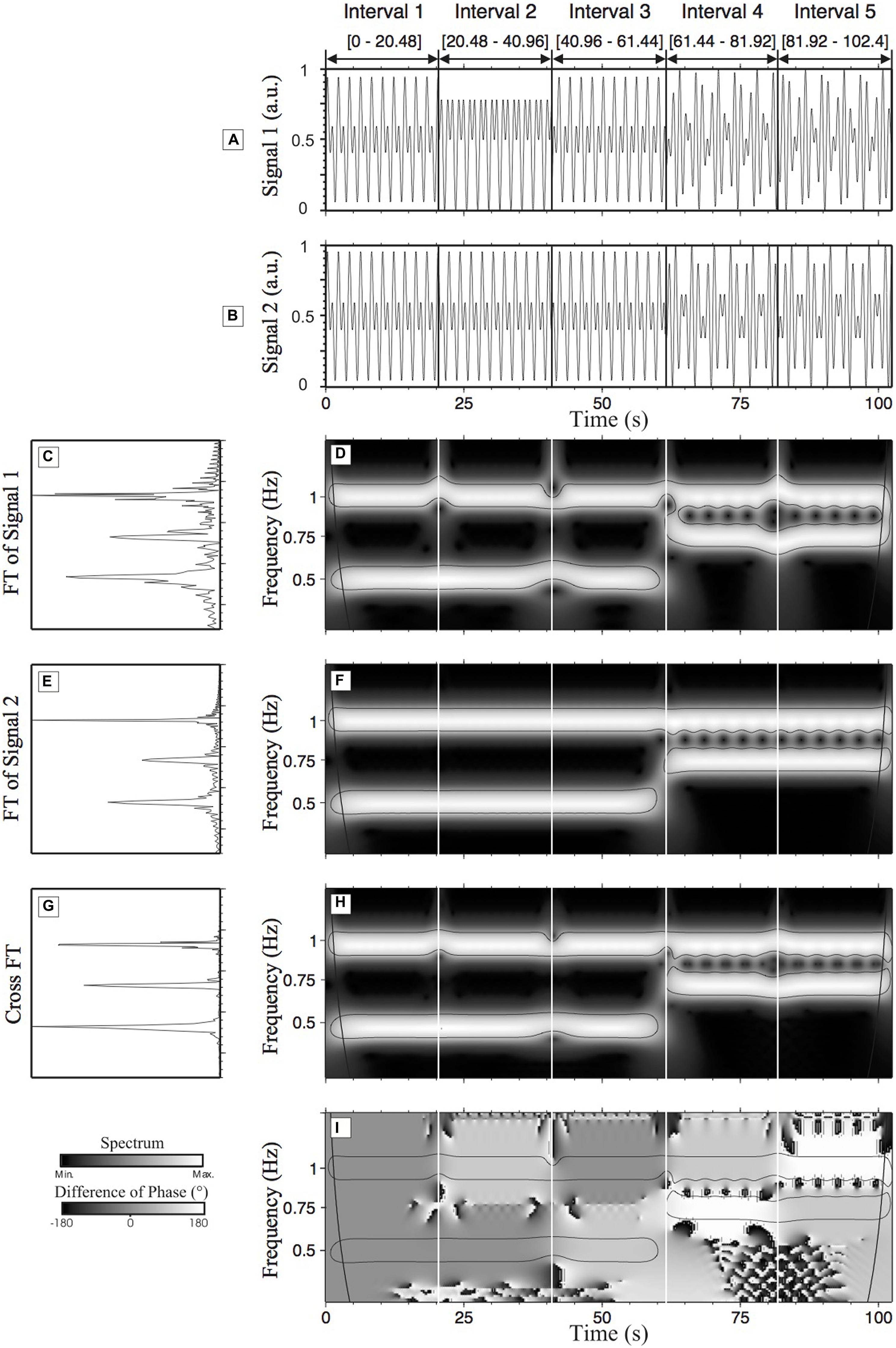
Here I repost the example given in the referenced tutorial. Two synthetic time-series were created. The two time-series, s1 (Figure 2A) and s2 (Figure 2B) have a duration of 102.4 s (with a sampling rate of 50 Hz). The amplitude of s1 and s2 is 1 arbitrary unit (a.u.). Both time-series have been divided into five intervals.

• For the first three intervals [0–61.44], the time-series are composed of a high frequency component at 1 Hz and a low frequency component at 0.5 Hz.
• For the last two intervals [61.44–102.4], the time-series are composed of a high frequency component (1 Hz) and an intermediate frequency component (0.75 Hz).
• 1st interval: characterized by a zero degree RP between s1 and s2 (the two time-series are identical in this interval).
• 2nd interval: the time-series s1 is characterized by a 90° phase lag in the high frequency component (1 Hz).
• 3rd interval: a 90° phase lag is applied on s1 in the low frequency component (0.5 Hz).
• 4th interval: a phase lag of 90° on the high frequency component and a phase lag of 180° on the intermediate frequency component are applied to s1.
• 5th interval: a phase lag of 180° on the high frequency component and of 90° on the intermediate frequency component are applied to s1 (see Table 1 for a summary of the changes made to s1).
• No phase lag exists in s2.

TABLE 1. Details of the phase lag and frequency modulations of s1.

FIGURE 1. Wavelet transform analysis and cross-wavelet transform (CWT) analysis of time-series (s1 and s2). (A,B) are the representations of s1 and s2, respectively; (C,E) show the normalized Fourier spectrum of (A,B), respectively. In both cases, we can observe one main peak at 1 Hz and two other peaks at 0.75 Hz and 0.5 Hz. (D,F) are WT spectra (scaleograms) of (A,B) respectively. These figures help to localize and quantify in terms of time of localization (time) and amplitude the frequency components previously identified in the Fourier spectra. In (D,F) two frequency components are present in the three first intervals of the time-series s1 and s2: one frequency at 1 Hz and one at 0.5 Hz. In the two last intervals, there are two frequencies: the frequency at 1 Hz, as in the three first intervals, and a new intermediate frequency at 0.75 Hz. (G) shows the cross-Fourier spectrum of (C,E). (H) Shows the cross-wavelet spectrum that is a representation of the common frequencies of (D,F) reflecting the local degree of interaction between the two analyzed time-series s1 and s2. (I) Shows the difference of phase of (A,B), i.e., the difference of phase between s1 and s2. The levels of gray permit us to visualize the associated relative phase (RP). a.u., arbitrary unit.

Discriminate the Properties of Time-Series

Following the statistical test described in Wavelet Transform, we can obtain what is usually known as the cone of influence, which is the region under the thin black lines in Figure 1.

Tools

MATLAB

MATLAB’s wavelet toolbox provides wcoherence for computing the cross-wavelet tranform. The key formula is

\[ \frac{| S(C_x^\ast(a,b) C_y(a,b) ) |^2}{S(| C_x(a,b) |^2)\cdot S(| C_y(a,b) |^2)} \]

where \( C_x(a,b) \) and \( C_y(a,b) \) denote the continuous wavelet transforms of x and y at scales a and positions b. The superscript * is the complex conjugate and S is a smoothing operator in time and scale.

Julia

Waiting for the magic to happen in ContinuousWavelets.jl.

1. This acronym is also used for continuous wavelet transform, to be distinguished from discrete wavelet transform. In MATLAB, the cwt function refers to continuous wavelet transform. ↩

2. There is a nice reference in the field of psychology, The relevance of the cross-wavelet transform in the analysis of human interaction – a tutorial. ↩