Fundamentals of Kinetic Theory#
Phase Space#
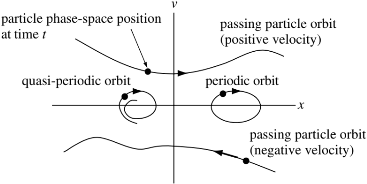
Consider a particle moving in a one-dimensional space and let the position of the particle be \(x = x(t)\) and the velocity of the particle be \(v = v(t)\). A way to visualize the \(x\) and \(v\) trajectories simultaneously is to plot these trajectories parametrically on a two-dimensional graph, where the horizontal coordinate is given by \(x(t)\) and the vertical coordinate is given by \(v(t)\). This x-v plane is called phase-space. The trajectory (or orbit) of several particles can be represented as a set of curves in phase-space. Examples of a few qualitatively different phase-space orbits are shown in the following figure.
 .
.
Particles in the upper half-plane always move to the right, since they have a positive velocity, while those in the lower half-plane always move to the left. Particles having exact periodic motion (e.g., \(x = A\cos t,\, v = −A\sin t\)) alternate between moving to the right and the left and so describe an ellipse in phase-space. Particles with quasi-periodic motions will have near-ellipses or spiral orbits. A particle that does not reverse direction is called a passing particle, while a particle confined to a certain region of phase-space (e.g., a particle with periodic motion) is called a trapped particle.
Distribution Function#
The fluid theory is the simplest description of a plasma; it is indeed fortunate that this approximation is sufficiently accurate to describe the majority of observed phenomena. There are some phenomena, however, for which a fluid treatment is inadequate. At any given time, each particle has a specific position and velocity. We can therefore characterize the instantaneous configuration of a large number of particles by specifying the density of particles at each point \(x, v\) in phase-space. The function prescribing the instantaneous density of particles in phase-space is called the distribution function and is denoted by \(f(x, v, t)\). Thus, \(f(x, v, t)\mathrm{d}x\mathrm{d}v\) is the number of particles at time \(t\) having positions in the range between \(x\) and \(x+\mathrm{d}x\) and velocities in the range between \(v\) and \(v+\mathrm{d}v\). As time progresses, the particle motion and acceleration causes the number of particles in these \(x\) and \(v\) ranges to change and so \(f\) will change. This temporal evolution of \(f\) gives a description of the system more detailed than a fluid description, but less detailed than following the trajectory of each individual particle. Using the evolution of \(f\) to characterize the system does not keep track of the trajectories of individual particles, but rather characterizes classes of particles having the same \(x, v\).
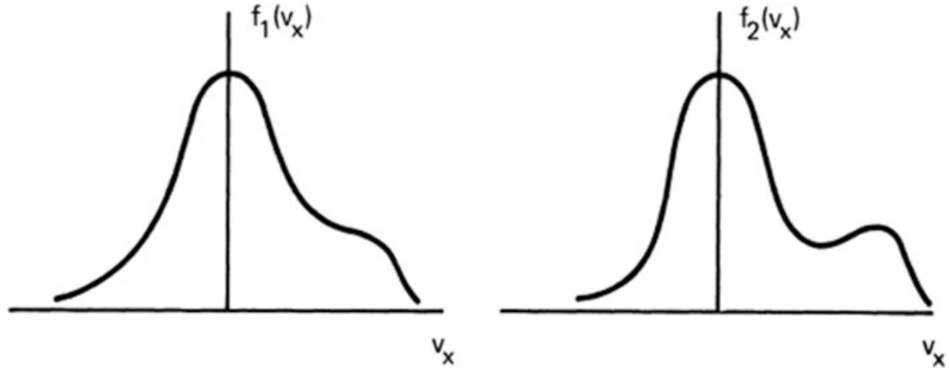
In fluid theory, the dependent variables are functions of only four independent variables: \(x, y, z,\) and \(t\). This is possible because the velocity distribution of each species is assumed to be Maxwellian everywhere and can therefore be uniquely specified by its bulk velocity \(\vec{U}\) and the temperature \(T\). Since collisions can be rare in high-temperature plasmas, deviations from thermal equilibrium can be maintained for relatively long times. As an example, consider two velocity distributions \(f_1(v_x)\) and \(f_2(v_x)\) in a one-dimensional system (figure below). These two distributions will have entirely different behaviors, but as long as the areas under the curves are the same, fluid theory does not distinguish between them.
When we consider velocity distributions in 3D, we have seven independent variables: \(f = f(\mathbf{r}, \mathbf{v}, t)\). By \(f(\mathbf{r}, \mathbf{v}, t)\), we mean that the number of particles per meter cubed at position \(\mathbf{r}\) and time \(t\) with velocity components between \(v_x\) and \(v_x + \mathrm{d}v_x\), \(v_y\) and \(v_y + \mathrm{d}v_y\), and \(v_z\) and \(v_z + \mathrm{d}v_z\) is
Moments of the distribution function#
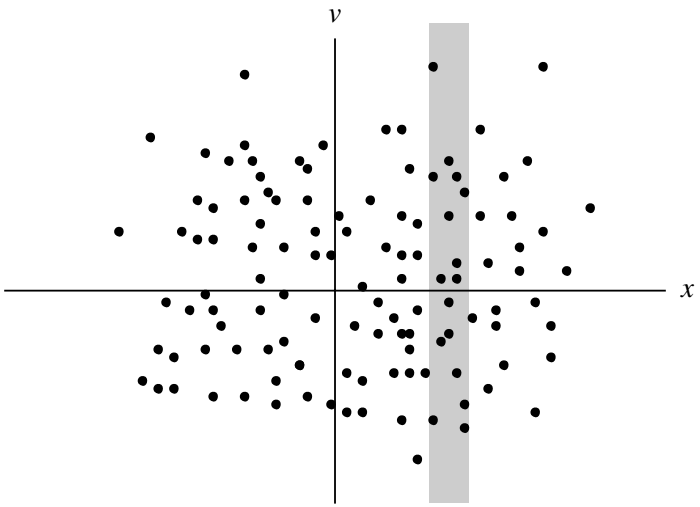
Let us count the particles in the shaded vertical strip in the above figure. The number of particles in this strip is the number of particles lying between \(x\) and \(x + \mathrm{d}x\), where \(x\) is the location of the left-hand side of the strip and \(x + \mathrm{d}x\) is the location of the right-hand side. The number of particles in the strip is equivalently defined as \(n(x, t)\mathrm{d}x\), where \(n(x)\) is the density of particles at \(x\). Thus we see that \(\int f(x, v)\mathrm{d}v = n(x)\) the transition from a phase-space description (i.e., \(x, v\) are independent variables) to a conventional description (i.e., only \(x\) is an independent variable) involves “integrating out” the velocity dependence to obtain a quantity (e.g., density) depending only on position. Since the number of particles is finite, and since \(f\) is a positive quantity, \(f\) must vanish as \(v\rightarrow\pm\infty\).
In three-dimension, the density is now a function of four scalar variables, \(n=n(\mathbf{r}, t)\), which is the integral of the distribution function over the velocity space:
Note that \(\mathrm{d}\mathbf{v}\) is not a vector; it stands for a three-dimensional volume element in velocity space. If \(f\) is normalized so that
Thus
is the probability that a randomly selected particle at position \(\mathbf{r}\) has the velocity \(\mathbf{v}\) at time \(t\). Using this point of view, we see that averaging over the velocities of all particles at \(x\) gives the mean velocity
Similarly, multiplying \(\hat{f}\) by \(mv^2/2\) and integrating over velocity will give an expression for the mean kinetic energy of all the particles. This procedure of multiplying \(f\) by various powers of \(\mathbf{v}\) and then integrating over velocity is called taking moments of the distribution function.
Note that \(\hat{f}\) is still a function of seven variables, since the shape of the distribution, as well as the density, can change with space and time. From (3), it is clear that \(\hat{f}\) has the dimensions \((\text{m}/\text{s})^{-3}\); and consequently, from (4), \(f\) has the dimensions \(\text{s}^3 \text{m}^{-6}\).
Maxwellian Distribution#
A particularly important distribution function is the Maxwellian:
where
This is the normalized form where \(\hat{f}_m\) is equivalent to probability: by using the definite integral
one easily verifies that the integral of \(\hat{f}_m\) over \(\mathrm{d}v_x \mathrm{d}v_y \mathrm{d}v_z\) is unity.
A common question being asked is:
Why do we see Maxwellian/Gaussian/normal distribution ubiquitously in nature?
Well, this is related to the central limit theorem in statistics: in many situations, when independent random variables are summed up, their properly normalized sum tends toward a normal distribution even if the original variables themselves are not normally distributed (e.g. a biased coin which give 95% head and 5% tail). In statistical physics, this is related to the fact that a Maxwellian distribution represents the state of a system with the highest entropy under the constraint of energy conservation.
There are several average velocities of a Maxwellian distribution that are commonly used. The root-mean-square velocity is given by
The average magnitude of the velocity \(|v|\), or simply \(\bar{v}\), is found as follows:
Since \(\hat{f}_m\) is isotropic, the integral is most easily done in spherical coordinates in v space. Since the volume element of each spherical shell is \(4\pi v^2 \mathrm{d}v\), we have
The definite integral has a value 1/2, found by integration by parts. Thus
The velocity component in a single direction, say \(v_x\), has a different average. Of course, \(\bar{v}_x\) vanishes for an isotropic distribution; but \(|\bar{v}_x|\) does not:
To summarize: for a Maxwellian,
For an isotropic distribution like a Maxwellian, we can define another function \(g(v)\) which is a function of the scalar magnitude of \(\mathbf{v}\) such that
For a Maxwellian, we see that
Note the difference between \(g(v)\) and a one-dimensional Maxwellian distribution \(f(v_x)\). Although \(f(v_x)\) is maximum for \(v_x=0\), \(g(v)\) is zero for \(v=0\). This is just a consequence of the vanishing of the volume in phase space for \(v=0\). Sometimes \(g(v)\) is carelessly denoted by \(f(v)\), as distinct from \(f(\mathbf{v})\); but \(g(v)\) is a different function of its argument than \(f(\mathbf{v})\) is of its argument. From (7), it is clear that \(g(v)\) has dimensions \(\text{s}/\text{m}^4\).
Gallery#
Isotropic Maxwellian distribution
Anisotropic (pancake) distribution
Beam
Crescent shape