Ion Distribution From MMS

This notebook shows how to create 2D slices of 3D particle data from FPI using PySPEDAS. pyspedas is the Python implementation of SPEDAS orginally coded in IDL. It is not as feature-complete as the IDL version.

Obtaining MMS FPI Data

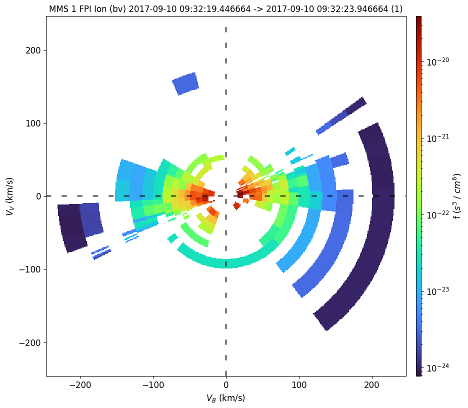
Here is a recorded bi-directional field-aligned beam of 0-300 eV ions observed by FPI. Due to a bug in the time argument of mms_part_slice2d, we currently need to specify the start and end time of the interval as a list.

from pytplot import time_double, time_string

time = "2017-09-10/09:32:20"
window = 4.
trange = [time_double(time)-window/2, time_double(time)+window/2]

time_string(trange)

---------------------------------------------------------------------------
ModuleNotFoundError                       Traceback (most recent call last)
Cell In[1], line 1
----> 1 from pytplot import time_double, time_string
      3 time = "2017-09-10/09:32:20"
      4 window = 4.

ModuleNotFoundError: No module named 'pytplot'

The data is downloaded automatically to the pydata folder under the current directory if not found.

from pyspedas.mms.particles.mms_part_slice2d import mms_part_slice2d

mms_part_slice2d(
    time=time,
    instrument="fpi",
    species="i",
    rotation="bv",
    erange=[0, 300],
    cmap="turbo",
)

Basic operations

To return the slice data structure instead of plotting, set the return_slice keyword to True:

the_slice = mms_part_slice2d(
    return_slice=True,
    time=time,
    instrument="fpi",
    species="i",
    rotation="bv",
    erange=[0, 300],
)

The slice is stored as a dictionary:

the_slice.keys()

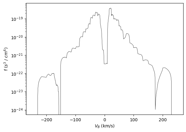
We can create 1D cuts through the 2D slice by specifying the velocity range:

(hyzhou: why is the unit still the same as in 2D/3D?)

from pyspedas.particles.spd_slice2d.slice1d_plot import plot

plot(the_slice, 'x', [-100, 100])  # summed from Vv=[-100, 100]

FPI ions with 2D interpolation

The data are rotated such that the x axis is parallel to B field and the bulk velocity defines the x-y plane, and plotted using 2D interpolation (data points within the specified theta or z-axis range are projected onto the slice plane and linearly interpolated onto a regular 2D grid). The default theta range is [-20, +20].

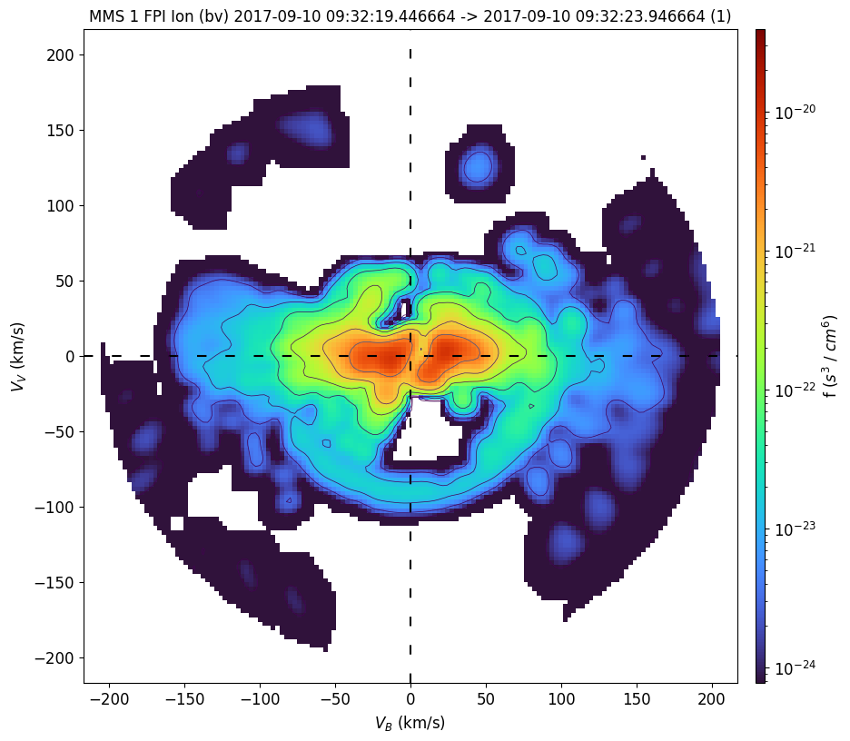
mms_part_slice2d(interpolation="2d", time=time, instrument="fpi", species="i", rotation="bv", erange=[0, 300], cmap="turbo")

slicemms2d = mms_part_slice2d(return_slice=True, interpolation="2d", time=time, instrument="fpi", species="i", rotation="bv", erange=[0, 300])

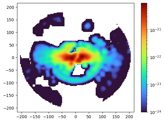
import matplotlib.pyplot as plt
import matplotlib.colors as colors
import numpy as np

plt.pcolormesh(slicemms2d["xgrid"], slicemms2d["ygrid"], slicemms2d["data"].T,
               norm=colors.LogNorm(1e-24, np.nanmax(slicemms2d["data"])),
               cmap="turbo")
plt.colorbar()
plt.show()