Blunt Body Problem in Hydrodynamics
At first sight, this seems to be an easy problem: there should be some kind of analytical solution given an ideal shape of the obstacle, say a cylinder in 2D or sphere in 3D. Unfortunately, there’re no such simple solutions.
The introduction here is taken from Time-Dependent Computation for Blunt Body Flows by D. FREUDENREICH’s master of engineering thesis.
Definition
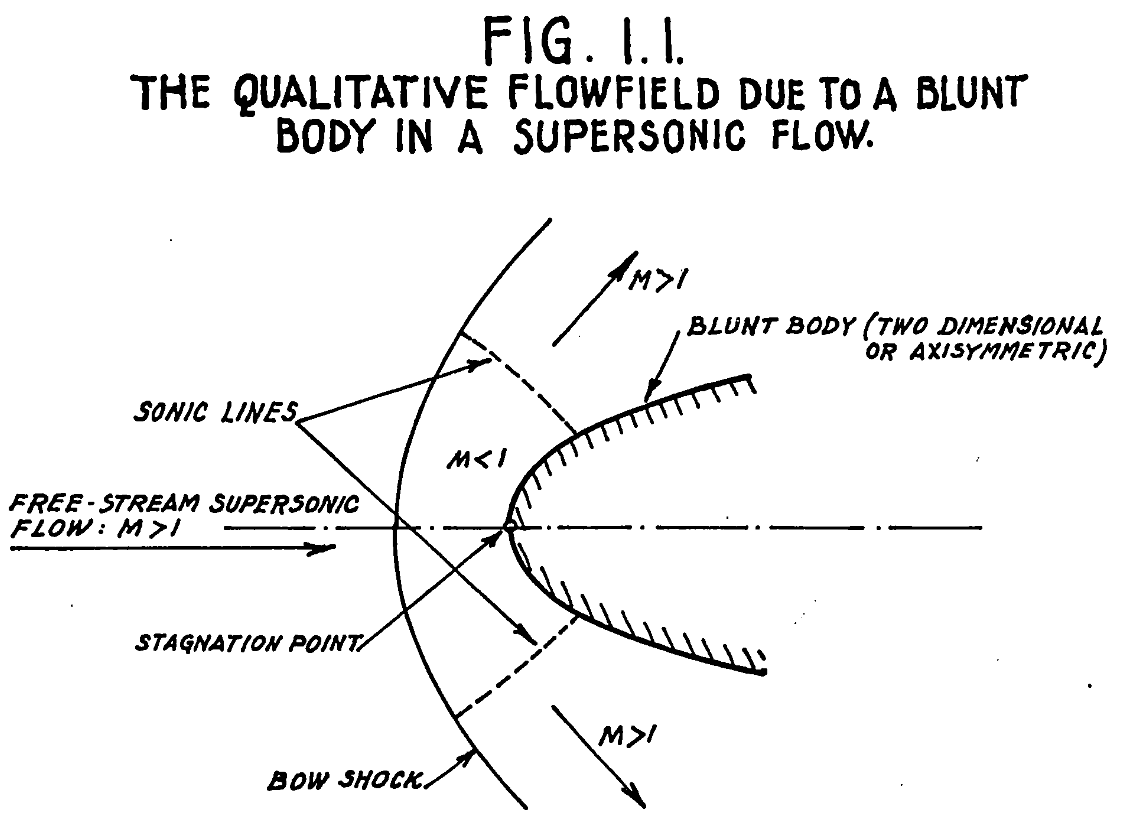
The blunt body problem consists of determining the flow field, including the location and shape of the bow shock formed, due to a supersonic flow around a body with a blunt leading edge.
The conservation laws which describe the motion of the flow are a set of nonlinear partial differential equations. The flow is supersonic ahead of the bow shock formed but subsonic behind it, up to sonic line, after which the flow is again supersonic, as shown in fig. 1.1; hence the problem is one of mixed supersonic-subsonic flows.
Another difficulty is that the boundaries in the problem are not completely defined, that is, only the shape of the body is known a priori. The other boundaries consisting of the bow shock and the sonic lines have to he determined as weIl as the flow properties in the region of flow.
The key thing to remember is that there is no analytical solution yet.
Classical Shock-Capturing Technique
It was not until G.Moretti and M.Abbett’s idea that this becomes computationally feasible. The time-dependency of the method is based on considering the conservation equations for the problem in their unsteady configuration. In this form the governing equations are hyperbolic with respect to time, which therefore makes the technique very well suited for the unified analysis of mixed subsonic-supersonic flows.
The ana1ysis is started by assuming an arbitrary shock profile AB, as shown in fig. 1.2.
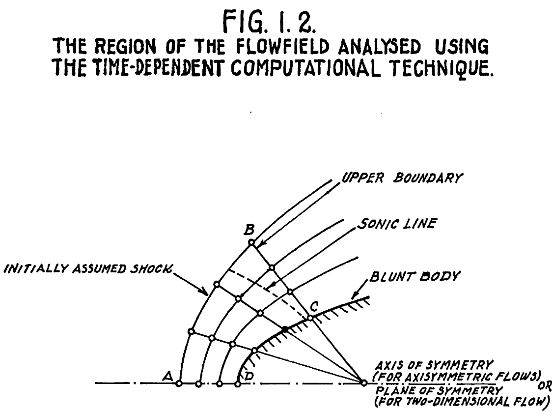
The region that is analysed is that part of the flow field which is bounded by the assumed shock, the body surface, the plane of symmetry (AD in fig. 1.2) and an arbitrary upper boundary which must be in the supersonic region of the flow, that is, downstream of the sonic 1ine. The reason that the upper boundary shou1d be “innnersed” in the supersonic part of the f1ow, is to ensure that no distrubances are propagated back into the region under consideration; since for supersonic flows, disturbances are only propagated downstream. Thus referring to fig. 1.2, the region of flow represented by ABCD is the one under consideration. This region is then divided into a network of points and the flow parameters inc1uding pressure, density and velocity are initia11y assumed for each point.
A time interva1 \( \Delta t \) is then considered and using a modified method of characteristics the shock shape and location are re-ca1cu1ated, as well as the flow parameters just behind the shock which must satisfy the Rankine-Hugoniot equations. Simi1ar1y on the body surface the flow variables are found using the same modified method of characteristics.
Having found the value of the flow parameters on the boundary points, that is, the shock and body points along AB and CD respectively in fig. 1.2, the new values of the dependent variables at the inner points between the two boundaries have to be determined. This is done by using the governing equations, which inc1ude the continuity equation, the momentum equation and the energy equation written in their unsteady form, that is, the partial time derivative \( \partial/\partial t \) of the different dependent variables is retained in the above mentioned equations. These equations are then written in a finite difference form and the new values of the flow variables at each mesh point can be determined.
Thus, the flow over the whole region ABCD can be calculated for a time step \( \Delta t \) from the initial1y assumed values of the flow parameters. The above procedure is then repeated for another time step using the previously obtained values of the dependent variables as initial values. The above is then again repeated and continued until no appreciable change in the flow variables is obtained between one time step and the other, at which stage the resu1ting flow pattern is said to be the steady state solution, having been reached from the unsteady flow configuration in an asymptotic manner with respect to time.
Initial Setup
A proper initial condition would speed up the computation process significantly. However, I believe any initial condition should converge to the same steady state solution.
Governing Equations
Compressible fluid dynamics? I don’t have time to go through the derivations, but it seems like classical finite difference method for solving the conservation equations. While the classical methods use central differences, the modern methods are almost all based on variations of upwind schemes.