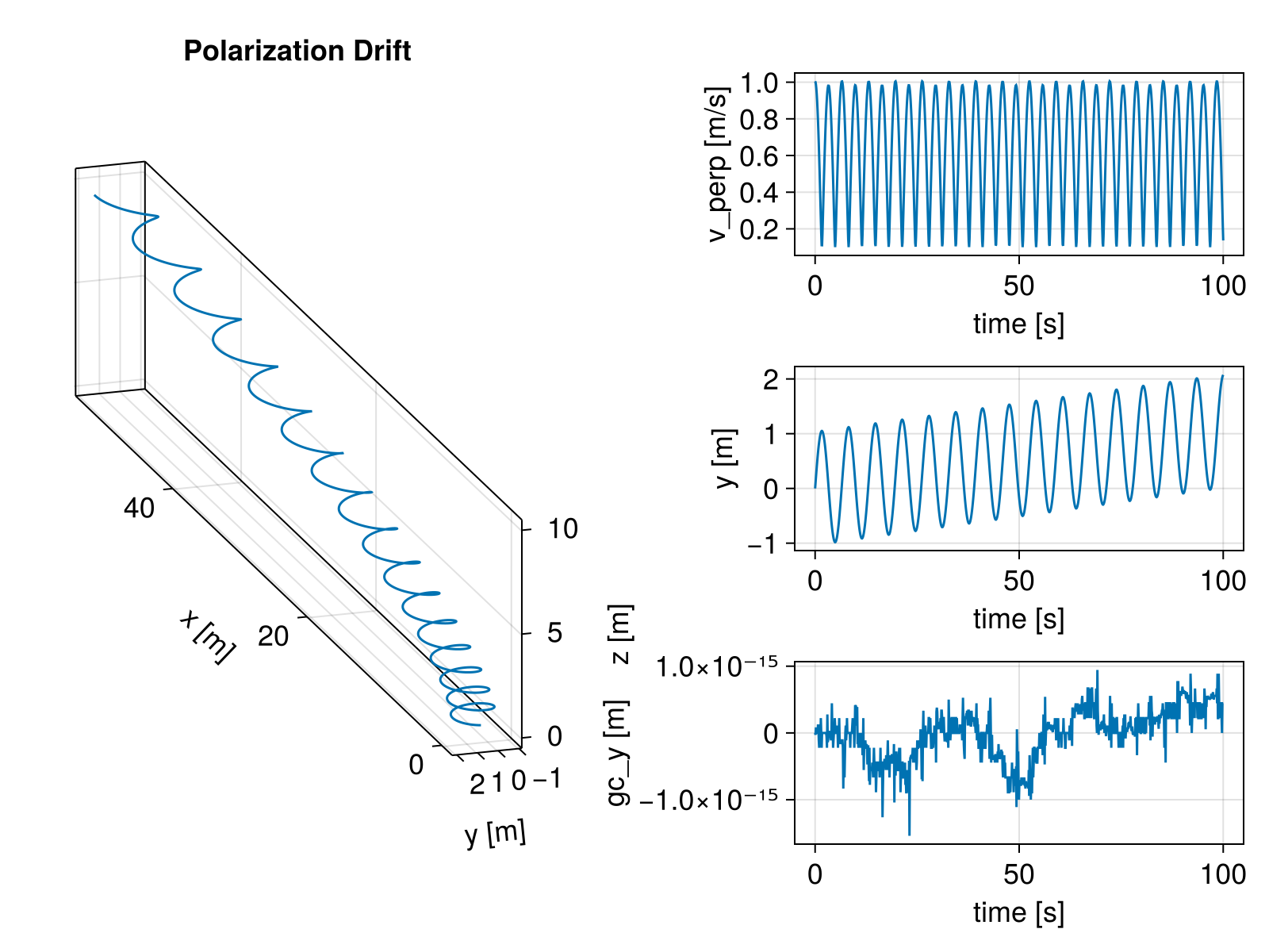
Polarization drift

This example demonstrates a single proton motion under time-varying E field. More theoretical details can be found in Time-Varying E Drift, and Fundamentals of Plasma Physics by Paul Bellan.

using TestParticle
using OrdinaryDiffEq
using StaticArrays
using CairoMakie

function uniform_B(x)
    return SA[0, 0, 1e-8]
end

function time_varying_E(x, t)
    # return SA[0, 1e-9*cos(0.1*t), 0]
    return SA[0, 1e-9*0.1*t, 0]
end

# Initial condition
stateinit = let x0 = [1.0, 0, 0], v0 = [0.0, 1.0, 0.1]
    [x0..., v0...]
end
# Time span
tspan = (0, 100)
param = prepare(time_varying_E, uniform_B, species=Proton)
prob = ODEProblem(trace!, stateinit, tspan, param)
sol = solve(prob, Vern9())
# Functions for obtaining the guiding center from actual trajectory
gc = get_gc(param)
v_perp(xu) = sqrt(xu[4]^2 + xu[5]^2)

# Visualization
f = Figure(size=(800, 600), fontsize=18)
ax1 = Axis3(f[1:3, 1],
   title = "Polarization Drift",
   xlabel = "x [m]",
   ylabel = "y [m]",
   zlabel = "z [m]",
   aspect = :data,
   azimuth = 0.9π,
   elevation = 0.1π
)
ax2 = Axis(f[1,2], xlabel = "time [s]", ylabel = "v_perp [m/s]")
ax3 = Axis(f[2,2], xlabel = "time [s]", ylabel = "y [m]")
ax4 = Axis(f[3,2], xlabel = "time [s]", ylabel = "gc_y [m]")

gc_y(t, x, y, z, vx, vy, vz) = (t, gc(SA[x, y, z, vx, vy, vz])[2])
v_perp(t, vy, vz) = (t, sqrt(vy^2 + vz^2))

lines!(ax1, sol, idxs=(1, 2, 3))
lines!(ax2, sol, idxs=(v_perp, 0, 5, 6))
lines!(ax3, sol, idxs=2)
lines!(ax4, sol, idxs=(gc_y, 0, 1, 2, 3, 4, 5, 6))

This page was generated using DemoCards.jl and Literate.jl.