Plot Functions
TestParticle.jl wraps types of AbstractODESolution from DifferentialEquations.jl. The plotting recipes for Plots.jl and Makie.jl work automatically for the particle tracing solutions.
Before using the plot recipes of Testparticle.jl, you need to import Makie package via using GLMakie or using CairoMakie, which depends on your choice for the backend. All plot recipes depend on Makie.jl.
Convention
By convention, we use integers to represent the 7 dimensions in the input argument idxs for all plotting methods:
| Component | Meaning |
|---|---|
| 0 | time |
| 1 | x |
| 2 | y |
| 3 | z |
| 4 | vx |
| 5 | vy |
| 6 | vz |
Basic recipe
The simplest usage is directly calling the plot or lines function provided by Makie. For example,
plot(sol, idxs=(1, 2, 3))The keyword argument idxs can be used to select the variables to be plotted; if not specified, it will plot the timeseries of x, y, z, vx, vy, vz. Please refer to Choose Variables for details.
If you want to plot a function of time, position or velocity, you can first define the function. For example,
Eₖ(t, vx, vy, vz) = (t, mₑ*(vx^2 + vy^2 + vz^2)/2)
lines(sol, idxs=(Eₖ, 0, 4, 5, 6))
will plot the kinetic energy as a function of x.
You can choose the plotting time span via the keyword argument tspan. For example,
lines(sol, tspan=(0, 1))The plots can be customized further:
f = Figure(size=(1200, 800), fontsize=18)
ax = Axis3(f[1,1],
    title = "Particle trajectory",
    xlabel = "X",
    ylabel = "Y",
    zlabel = "Z",
)

plot!(sol, idxs=(1, 2, 3))
Multiple particle trajectories saved as the type EnsembleSolution is also supported by the Makie recipe.
Advanced recipe
We currently rely on the Makie recipe implemented in DiffEqBase.jl. This recipe depends on an experimental API introduced in Makie v0.20, which may be unstable and contains bugs. Once it becomes more stabilized with bug fixes, we will recover the interactive widgets support, e.g. orbit and monitor.
orbit
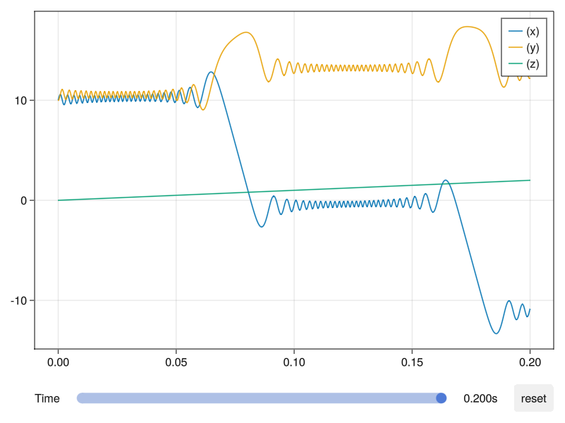
The slider can control the time span, and the maximum of time span will be displayed on the right of the slider.
The reset button can reset the scale of lines when the axis limits change. When you drag the slider, clicking reset button will reset the axis limits to fit the data.
monitor
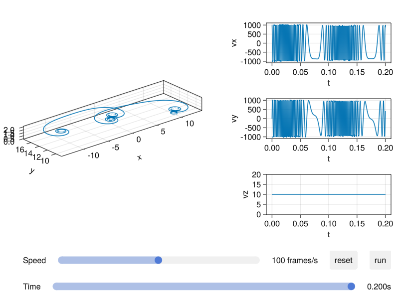
After first click of the run button, the evolution of the orbit will be displayed from the beginning. For other times, it will start from the time set by the time slider. The functionality of reset button is the same as above.
The time slider controls the time span. The speed slider controls the speed of the animation.