Energy Conservation

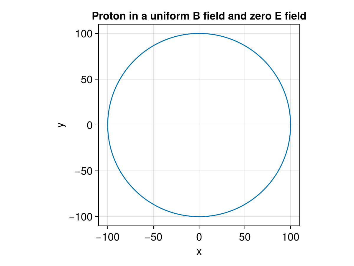
This example demonstrates the energy conservation of a single proton motion in two cases. The first one is under a uniform B field and zero E field. The second on is under a zero B field and uniform E field.

using TestParticle
using OrdinaryDiffEq
using StaticArrays
using LinearAlgebra: ×
using CairoMakie

const B₀ = 1e-8 # [T]
const E₀ = 3e-2 # [V/m]

"f2"
function location!(dx, v, x, p::TestParticle.TPTuple, t)
   dx .= v
end

"f1"
function lorentz!(dv, v, x, p::TestParticle.TPTuple, t)
   q2m, E, B = p
   dv .= q2m*(E(x, t) + v × (B(x, t)))
end

### Initialize field

function uniform_B(x)
   return SA[0, 0, B₀]
end

function uniform_E(x)
   return SA[E₀, 0.0, 0.0]
end

function zero_B(x)
   return SA[0.0, 0.0, 0.0]
end

function zero_E(x)
   return SA[0.0, 0.0, 0.0]
end

"Check energy conservation."
E(dx, dy, dz) = 1 // 2 * (dx^2 + dy^2 + dz^2)

### Initialize particles

x0 = [0.0, 0, 0]
v0 = [0.0, 1e2, 0.0]
stateinit = [x0..., v0...]
tspan_proton = (0.0, 2000.0);

Uniform B field and zero E field

param_proton = prepare(zero_E, uniform_B, species=Proton)

### Solve for the trajectories

prob_p = DynamicalODEProblem(lorentz!, location!, v0, x0, tspan_proton, param_proton)

Ωᵢ = TestParticle.qᵢ * B₀ / TestParticle.mᵢ
Tᵢ = 2π / Ωᵢ
println("Number of gyrations: ", tspan_proton[2] / Tᵢ)

sol = solve(prob_p, ImplicitMidpoint(), dt = Tᵢ/15)

f = Figure(fontsize=18)
ax = Axis(f[1, 1],
    title = "Proton in a uniform B field and zero E field",
    xlabel = "x",
    ylabel = "y",
    aspect = 1,
)

lines!(ax, sol, idxs=(1, 2))

Zero B field and uniform E field

param_proton = prepare(uniform_E, zero_B, species=Proton)

# acceleration, [m/s²]
a = param_proton[1] * E₀
# predicted final speed, [m/s]
v_final_predict = a * tspan_proton[2]
# predicted travel distance, [m/s]
d_final_predict = 0.5 * tspan_proton[2] * v_final_predict
# predicted energy gain, [eV]
E_predict = E₀ * d_final_predict

prob_p = DynamicalODEProblem(lorentz!, location!, v0, x0, tspan_proton, param_proton)

sol = solve(prob_p, Vern6())

energy = map(x -> E(x[1:3]...), sol.u) .* TestParticle.mᵢ;

Predicted final speed

predicted final speed: 5.744086746808526e9 [m/s]

Simulated final speed

simulated final speed: 5.744086746808613e9 [m/s]

Predicted travel distance

predicted travel distance: 5.744086746808526e12 [m]

Simulated travel distance

simulated travel distance: 5.744086746768604e12 [m]

Predicted final energy

predicted energy gain: 1.723226024042558e11 [eV]

Simulated final energy

simulated final energy: 1.7232260240426102e11 [eV]

This page was generated using DemoCards.jl and Literate.jl.