Curl-B drift

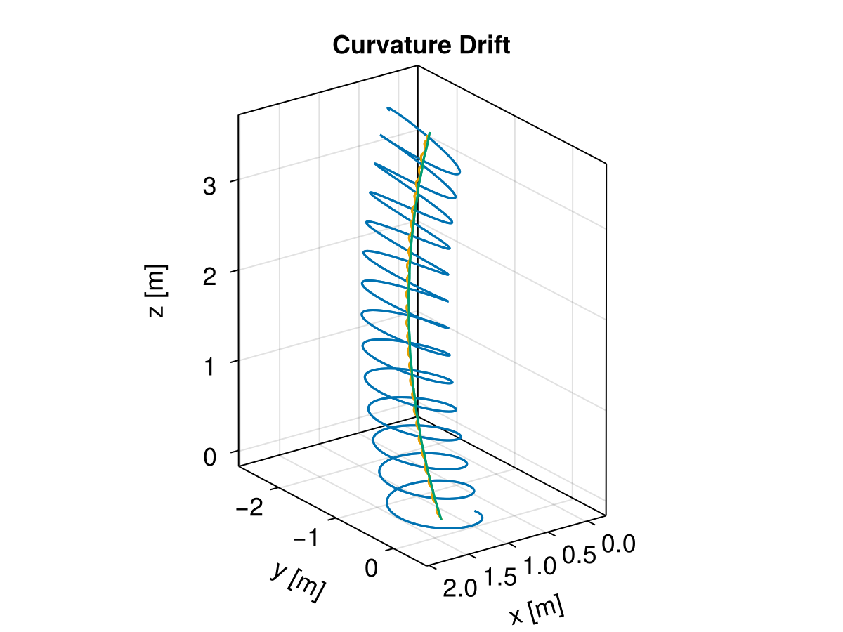
This example demonstrates a single proton motion under a vacuum non-uniform B field with gradient and curvature. Similar to the magnetic field gradient drift, analytic calculation should include both of the gradient drift and the curvature drift. More theoretical details can be found in Curvature Drift and Computational Plasma Physics by Toshi Tajima.

using TestParticle
using TestParticle: get_gc
using OrdinaryDiffEq
using StaticArrays
using LinearAlgebra: normalize, norm, ×, ⋅
using ForwardDiff: gradient, jacobian
using CairoMakie

function curved_B(x)
    # satisify ∇⋅B=0
    # B_θ = 1/r => ∂B_θ/∂θ = 0
    θ = atan(x[3] / (x[1] + 3))
    r = sqrt((x[1] + 3)^2 + x[3]^2)
    return SA[-1e-7*sin(θ)/r, 0, 1e-7*cos(θ)/r]
end

function zero_E(x)
    return SA[0, 0, 0]
end

abs_B(x) = norm(curved_B(x))  # |B|

# Trace the orbit of the guiding center using analytical drifts
function trace_gc!(dx, x, p, t)
    q2m, E, B, sol = p
    xu = sol(t)
    gradient_B = gradient(abs_B, x)  # ∇|B|
    Bv = B(x)
    b = normalize(Bv)
    v_par = (xu[4:6] ⋅ b).*b  # (v⋅b)b
    v_perp = xu[4:6] - v_par
    Ω = q2m*norm(Bv)
    κ = jacobian(B, x)*Bv  # B⋅∇B
    # v⟂^2*(B×∇|B|)/(2*Ω*B^2) + v∥^2*(B×(B⋅∇B))/(Ω*B^3) + (E×B)/B^2 + v∥
    dx[1:3] = norm(v_perp)^2*(Bv × gradient_B)/(2*Ω*norm(Bv)^2) +
        norm(v_par)^2*(Bv × κ)/Ω/norm(Bv)^3 + (E(x) × Bv)/norm(Bv)^2 + v_par
end

# Initial conditions
stateinit = let x0 = [1.0, 0.0, 0.0], v0 = [0.0, 1.0, 0.1]
    [x0..., v0...]
end
# Time span
tspan = (0, 40)
# Trace particle
param = prepare(zero_E, curved_B, species=Proton)
prob = ODEProblem(trace!, stateinit, tspan, param)
sol = solve(prob, Vern9())
# Functions for obtaining the guiding center from actual trajectory
gc = get_gc(param)
gc_x0 = gc(stateinit)
prob_gc = ODEProblem(trace_gc!, gc_x0, tspan, (param..., sol))
sol_gc = solve(prob_gc, Tsit5(); save_idxs=[1,2,3])

# Numeric and analytic results
f = Figure(fontsize=18)
ax = Axis3(f[1, 1],
   title = "Curvature Drift",
   xlabel = "x [m]",
   ylabel = "y [m]",
   zlabel = "z [m]",
   aspect = :data,
   azimuth = 0.3π,
)

gc_plot(x, y, z, vx, vy, vz) = (gc(SA[x, y, z, vx, vy, vz])...,)

lines!(ax, sol, idxs=(1, 2, 3))
lines!(ax, sol, idxs=(gc_plot, 1, 2, 3, 4, 5, 6))
lines!(ax, sol_gc, idxs=(1, 2, 3))

for i in 1:3
    ##TODO: wait for https://github.com/MakieOrg/Makie.jl/issues/3623 to be fixed!
    ax.scene.plots[9+2*i-1].color = Makie.wong_colors()[i]
end

This page was generated using DemoCards.jl and Literate.jl.