Analytical magnetosphere

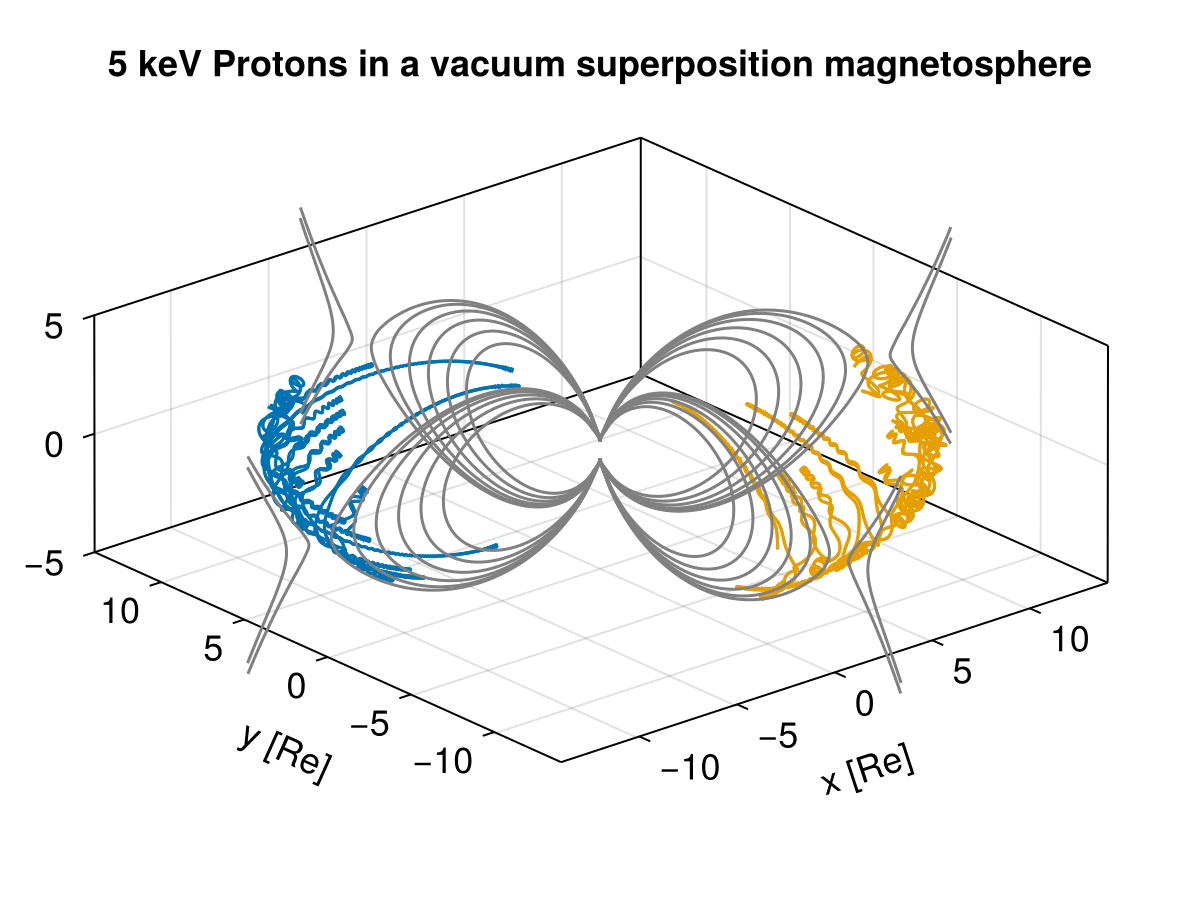
This demo shows how to trace particles in a vacuum superposition of a dipolar magnetic field $\mathbf{B}_D$ with a uniform background magnetic field $\mathbf{B}_\mathrm{IMF}$. In this slightly modified dipole field, magnetic null points appear near 14 Earth's radii, and the particle orbits are also distorted from the idealized motions in Demo: magnetic dipole.

using TestParticle
using TestParticle: getB_dipole, getE_dipole, sph2cart, mᵢ, qᵢ, c, Rₑ
using OrdinaryDiffEq
using StaticArrays
using FieldTracer
using CairoMakie

function getB_superposition(xu)
   getB_dipole(xu) + SA[0.0, 0.0, -10e-9]
end

"Boundary condition check."
function isoutofdomain(u, p, t)
   rout = 18Rₑ
   if (u[1]^2 + u[2]^2 + u[3]^2) < (1.1Rₑ)^2 ||
      abs(u[1]) > rout || abs(u[2]) > rout || abs(u[3]) > rout
      return true
   else
      return false
   end
end

"Set initial conditions."
function prob_func(prob, i, repeat)
   # initial particle energy
   Ek = 5e3 # [eV]
   # initial velocity, [m/s]
   v₀ = sph2cart(c*sqrt(1-1/(1+Ek*qᵢ/(mᵢ*c^2))^2), 0.0, π/4)
   # initial position, [m]
   r₀ = sph2cart(13*Rₑ, π*i, π/2)

   prob = remake(prob; u0 = [r₀..., v₀...])
end

# obtain field
param = prepare(getE_dipole, getB_superposition)
stateinit = zeros(6) # particle position and velocity to be modified
tspan = (0.0, 2000.0)
trajectories = 2

prob = ODEProblem(trace!, stateinit, tspan, param)
ensemble_prob = EnsembleProblem(prob; prob_func, safetycopy=false)

# See https://docs.sciml.ai/DiffEqDocs/stable/basics/common_solver_opts/
# for the solver options
sols = solve(ensemble_prob, Vern9(), EnsembleSerial(); reltol=1e-5,
   trajectories, isoutofdomain, dense=true, save_on=true)

### Visualization

f = Figure(fontsize=18)
ax = Axis3(f[1, 1],
   title = "5 keV Protons in a vacuum superposition magnetosphere",
   xlabel = "x [Re]",
   ylabel = "y [Re]",
   zlabel = "z [Re]",
   aspect = :data,
   limits = (-14, 14, -14, 14, -5, 5)
)

invRE = 1 / Rₑ

for (i, sol) in enumerate(sols)
   l = lines!(ax, sol, idxs=(1, 2, 3))
   ##TODO: wait for https://github.com/MakieOrg/Makie.jl/issues/3623 to be fixed!
   scale!(ax.scene.plots[9+2*i-1], invRE, invRE, invRE)
   ax.scene.plots[9+2*i-1].color = Makie.wong_colors()[i]
end

# Field lines
function get_numerical_field(x, y, z)
   bx = zeros(length(x), length(y), length(z))
   by = similar(bx)
   bz = similar(bx)

   for i in CartesianIndices(bx)
      pos = [x[i[1]], y[i[2]], z[i[3]]]
      bx[i], by[i], bz[i] = getB_superposition(pos)
   end

   bx, by, bz
end

function trace_field!(ax, x, y, z, unitscale)
   bx, by, bz = get_numerical_field(x, y, z)

   zs = 0.0
   nr, nϕ = 8, 4
   dϕ = 2π / nϕ
   for r in range(8Rₑ, 16Rₑ, length=nr), ϕ in range(0, 2π-dϕ, length=nϕ)
      xs = r * cos(ϕ)
      ys = r * sin(ϕ)

      x1, y1, z1 = FieldTracer.trace(bx, by, bz, xs, ys, zs, x, y, z; ds=0.1, maxstep=10000)

      lines!(ax, x1.*unitscale, y1.*unitscale, z1.*unitscale, color=:gray)
   end
end

x = range(-18Rₑ, 18Rₑ, length=50)
y = range(-18Rₑ, 18Rₑ, length=50)
z = range(-18Rₑ, 18Rₑ, length=50)

trace_field!(ax, x, y, z, invRE)

This page was generated using DemoCards.jl and Literate.jl.