Incompressible Fluid Solver

Fluid simulation in industry focuses mostly on incompressible solvers. Mathematically incompressible fluids have simpler expressions and can be solved numerically in an efficient way. Here I am trying to learn some of the basic ideas and tricks, following the book Fluid Simulation for Computer Graphics, 2nd Edition and the excellent implementation. This is also a great opportunity for me to practice C++.

Eulerian approach is much easier in numerically approximating the spatial derivatives.

Semi-Lagrangian method is generally used for advection in solving the incompressible fluids numerically, because it's fast and often unconditionally stable.

Euler Equation

$\begin{aligned} \frac{D\mathbf{u}}{Dt} + \frac{1}{\rho}\nabla p &= \mathbf{g}\\ \nabla\cdot\mathbf{u} &= 0 \end{aligned}$

Splitting Method

With operator splitting, we'll work out methods for solving these simpler equations:

$\begin{aligned} \frac{Dq}{Dt} &= 0 \qquad (\text{advection}), \\ \frac{\partial \mathbf{u}}{\partial t} &= \mathbf{g} \qquad (\text{body forces}), \\ \frac{\partial \mathbf{u}}{\partial t} + \frac{1}{\rho}\nabla p &= 0 \qquad (\text{pressure}) \\ \text{such that}\, \nabla\cdot\mathbf{u} &= 0 \qquad (\text{incompressibility}) \end{aligned}$

Basic fluid algorithm:

• Start with an initial divergence-free velocity field $\mathbf{u}^0$

• For time step $n=0,1,2,...$

  • Determine a good time step $\Delta t$ to go from time $t_n$ to $t_{n+1}$.

  • Set $\mathbf{u}^A = \text{advect}(\mathbf{u}^n,\Delta t, \mathbf{u}^n)$.

  • Add $\mathbf{u}^B = \mathbf{u}^A + \Delta \mathbf{g}$.

  • Set $\mathbf{u}^{n+1} = \text{project}(\mathbf{u}^B,\Delta t)$.

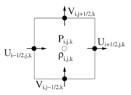
MAC Grid

In the early days of computational fluid dynamics, Harlow and Welch introduced the marker-and-cell (MAC) method method for solving incompressible flow problems. One of the fundamental innovations of this paper was a new grid structure that makes for avery effective algorithm for enforcing incompressibility, though it may seem inconvenient for everything else.

The so-called MAC grid is a staggered grid, i.e., a grid where the different variables are stored at different locations. (I remember there is another name of staggered grid after people doing MHD for EM field, but it's basically the same thing.) The raison d'être of the MAC grid is that the staggering makes accurate central differences robust.

Level Set Method

This part needs more complete info!

Some geometric problems are extremely common in fluid solvers:

• When is a point inside a solid?

• What is the closest point on the surface of some geometry?

• How do we extrapolate values from one region into another?

When I wrote my simple field tracer in Julia, I spent some time on the first query especially for 1D and 2D.

The first query above suggests the right approach is implicit surfaces. While there are potentially a lot of ways to generalize this, we will focus on the case where we have a continuous scalar function φ(x,y,z) which defines the geometry as follows:

• a point x is outside the geometry when φ(x) > 0,

• it’s inside the geometry when φ(x) < 0, and

• a point x is on the surface when φ(x) = 0.

In some other contexts within computer graphics, the convention may be reversed (the “outside” is the negative region) or a threshold value otherthan zero could be used, but this is usually the way we do it in fluid simulation.

Signed distance function (SDF): the gradient of the function is exactly unit-length normal on the surface.

level set: a signed distance function that has been sampled on a grid.

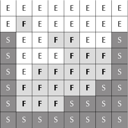
A two-dimensional example of a voxelized fluid domain. F stands for fluid, S for solid, and E for empty.

Advection

In the step of advection,

$\frac{D q}{Dt} = 0,$

we will encapsulate this in a numerical scheme

$\mathbf{u}^A = \text{advect}(\mathbf{u}^n,\Delta t, q^n)$

It bears repeating here: advection should only be called with a divergence-free velocity field $\mathbf{u}$, i.e., one meeting the incompressibility constraint, which also satisfies the required boundary conditions.

Projection

The heart of this scheme is to make this fluid incompressible and simultaneously enforce boundary conditions. The implementation of

$\mathbf{u}^{n+1} = \text{project}(\mathbf{u}^B,\Delta t)$

is the central topic.

The project routine will subtract the pressure gradient from the intermediate velocity field $\mathbf{u}$,

$\mathbf{u}^{n+1} = \mathbf{u}^n - \Delta t \frac{1}{\rho}\nabla p,$

so that the result satisfies incompressibility inside the fluid

$\nabla\cdot\mathbf{u} = 0,$

and satisfies the solid wall boundary conditions

$\mathbf{u}^{n+1}\cdot\widehat{n} = \mathbf{u}_{\text{solid}}\cdot\widehat{n}\qquad \text{at solid boundaries,}$

while also respecting the free surface boundary condition that pressure be zero there:

$p = 0\qquad \text{at free surfaces.}$

Without further ado, here are the formulas for the pressure update in two dimensions, using the central difference approximations for $\partial p/\partial x$ and $\partial p/\partial y$:

$\begin{aligned} u_{i+1/2,j}^{n+1} = u_{i+1/2,j}^n - \Delta t \frac{1}{\rho}\frac{p_{i+1,j} - p_{i,j}}{\Delta x} \\ u_{i,j+1/2}^{n+1} = u_{i,j+1/2}^n - \Delta t \frac{1}{\rho}\frac{p_{i,j+1} - p_{i,j}}{\Delta x} \end{aligned}$

One of the trickiest parts of writing a correct pressure solve is keeping track of which velocity and pressure samples are "active", so it's good to keep this in mind or perhaps refer to a diagram near you while you program. For the voxelized fluid model, fluid-containing voxels have an unknown pressure to be solved for (at which point it is valid), solid voxels do not have a valid pressure, and empty voxels have a valid pressure that’s already fixed at zero.

For the free surface boundary condition, we set the pressures in empty voxels to zero.

For the solid wall boundary condition on a MAC grid, where the staggered velocity components exactly line up with the solid surfaces, both in position and normal, we can go one step beyond the pressure gradient update and directly set the fluid velocity components on solid voxel faces adjacent to fluid equal to the solid velocity there. We can even think of this as an extension of the pressure gradient update by conceptually including a ghost value for pressure inside the solid voxel. For example, if the u-component of velocity at $(i+1/2,j,k)$ is between a solid voxel at $(i,j,k)$ and a fluid voxel at $(i+1,j,k)$, then setting

$u_{i+1/2,j,k}^{n+1} = u_{i+1/2,j,k}^{\text{solid}}$

is compatible with the usual pressure gradient update

$u_{i+1/2,j,k}^{n+1} = u_{i+1/2,j,k}^n - \Delta t \frac{1}{\rho}\frac{p_{i+1,j,k} - p_{i,j,k}^{\text{ghost}}}{\Delta x}$

as long as the ghost pressure in (i,j,k) satisfies

$p_{i,j,k}^{\text{ghost}} = p_{i+1,j,k} - \frac{\rho\Delta x}{\Delta t}(u_{i+1/2,j,k} - u_{i+1/2,j,k}^{\text{solid}}).$

More generally, this corresponds to

$\frac{\Delta t}{\rho}\nabla p\cdot\widehat{n} = (\mathbf{u} - \mathbf{u}^{\text{solid}})\cdot\widehat{n},$

i.e. when solving for pressure, the solid boundary condition amounts to specifying the normal derivative of pressure, $\partial p/\partial \widehat{n} = \nabla p\cdot\widehat{n}$, rather than the value of pressure.

Boundary	Type
Free surface	Dirichlet
Solid wall	Neumann

Boundary conditions can be complicated and are the usual culprit when bugs show up.

The pressure equations

Recall that we want the final velocity, $\mathbf{u}^{n+1}$ to be divergence-free inside the fluid. To find the pressure that achieves this, we simply substitute the pressure-update formulas for $\mathbf{u}^{n+1}$ into the divergence formula, which gives us a linear equation for each fluid grid cell, with pressures as unknowns.

In 2D,

$\frac{\Delta t}{\rho}\Big( \frac{4p_{i,j} - p_{i+1,j} - p_{i,j+1} - p_{i-1,j} - p_{i,j-1}}{\Delta x^2}\Big) = - \Big( \frac{u_{i+1/2,j} - u_{i-1/2,j}}{\Delta x} + \frac{v_{i,j+1/2} - v_{i,j-1/2}}{\Delta x} \Big)$

and in 3D,

$\frac{\Delta t}{\rho}\Big( \frac{6p_{i,j,k} - p_{i+1,j,k} - p_{i,j+1,k} - p_{i,j,k+1} - p_{i-1,j,k} - p_{i,j-1,k} - p_{i,j,k-1}} {\Delta x^2}\Big) = - \Big( \frac{u_{i+1/2,j,k} - u_{i-1/2,j,k}}{\Delta x} + \frac{v_{i,j+1/2,k} - v_{i,j-1/2,k}}{\Delta x} + \frac{v_{i,j,k+1/2} - v_{i,j,k-1/2}}{\Delta x} \Big)$

which are the numerical approximations to the Poisson problem

$\Delta t/\rho \nabla\cdot\nabla p = -\nabla\cdot\mathbf{u}.$

If a fluid grid cell is at the boundary, recall that the new velocities on the boundary faces involve pressures outside the fluid that we have to define through boundary conditions: we need to use that here. For example, if grid cell $(i, j+1)$ is an air cell, then we replace $p_{i,j+1}$ with zero. If grid cell $(i+1,j)$ is a solid cell, then we replace $p_{i+1,j}$ with the value we compute from the boundary condition there, as in Eq.(13). Assuming $(i−1, j)$ and $(i, j−1)$ are fluid cells, this would reduce the equation to the following:

$\frac{\Delta t}{\rho}\Big( \frac{3p_{i,j} - p_{i-1,j} - p_{i,j-1}}{\Delta x^2}\Big) = - \Big( \frac{u_{i+1/2,j} - u_{i-1/2,j}}{\Delta x} + \frac{v_{i,j+1/2} - v_{i,j-1/2}}{\Delta x} \Big) + \Big( \frac{u_{i+1/2,j} - u_{\text{solid}}}{\Delta x} \Big).$

Many observations can be made from this form.

Putting it in matrix-vector form

We have now defined a large system of linear equations for the unknown pressure values. We can conceptually think of it as a large coefficient matrix, $\overleftrightarrow{A}$, times a vector consisting of all pressure unknowns, $\mathbf{p}$, equal to a vector consisting of the negative divergences in each fluid grid cell, $\mathbf{b}$ (with appropriate modifidcations at solid wall boundaries):

$\overleftrightarrow{A}\mathbf{p} = \mathbf{b}.$

In practice, we don't need to store $\overleftrightarrow{A}$ directly as a matrix, because it is sparse, symmetric and pentadiagonal. Let $A_{(i,j,k),(i+1,j,k)}$ be the coefficient of $p_{i+1,j,k}$ in the equation for grid cell $(i,j,k)$. In two dimensions, we will store three numbers at every grid cell: the diagonal entry $A_{(i,j),(i,j)}$ and the entries for the neighboring cells in the positive directions $A_{(i,j),(i+1,j)}$ and $A_{(i,j),(i,j+1)}$.

The Conjugate Gradient Algorithm

The method introduced here is called MICCG(0),or more fully Modified Incomplete Cholesky Conjugate Gradient,Level Zero.

One of the many properties that $\overleftrightarrow{A}$ has is that it is symmetric positive definite (SPD). Technically this means that $\overleftrightarrow{A}$ is symmetric and $\mathbf{q}^TA\mathbf{q} > 0$ for any non-zero vector $\mathbf{q}$, or equivalently that its eigenvalues are all positive.

A might just be symmetric positive semi-definite, meaning that $\mathbf{q}^TA\mathbf{q} \ge 0$ (with zero achieved for some non-zero vector $\mathbf{q}$). If there is some fluid region entirely surrounded by solid walls, with no empty air cells, then A will not be strictly positive definite. In that case, A is singular in fact — it doesn’t have an inverse. That doesn’t necessarily mean there isn’t a solution, however. If the divergences (the right-hand side) satisfy a compatibility condition then life is good and there is a solution. The compatibility condition is simply that the velocities of the solid walls are compatible with the fluid contained within being incompressible — i.e., the fluid-solid boundary faces have wall velocities that add up to zero, so that the flow in is balanced by the flow out. In fact, not only will there be a solution, but there are infinitely many solutions! You can take any solution for pressure and add an arbitrary constant to it and get another solution, it turns out. However, when we take the pressure gradient for the velocity update, the constant term is annihilated so we don’t actually care which solution we get. They’re all good.

Projection

The project($\Delta t, \mathbf{u}$) routine does the following:

• Calculate the negative divergence $b$ (the right-hand side) with modifications at solid wall boundaries.

• Set the entries of $A$ (stored in $Adiag$, etc.).

• Construct the preconditioner (either MIC(0) for single threaded solves,or a more complicated domain decomposition set up for parallel solves).

• Solve $Ap = b$ with PCG.

• Compute the new velocities $\mathbf{u}^{n+1}$ according to the pressure-gradient update to $\mathbf{u}$.

There is a reason why this routine is called projection. If you recall from your linear algebra, a projection is a special type of linear operator such that if you apply it twice, you get the same result as applying it once. For example, a matrix $P$ is a projection if $P^2= P$. It turns out that our transformation from $\mathbf{u}^n$ to $\mathbf{u}^{n+1}$ is indeed a linear projection.^[1]

[1]	Technically speaking, if we have non-zero solid wall velocities then this is an affine transformation rather than a linear one, but it still is a projection. For the purpose of simplicity, we'll ignore this case here.

If you want, you can trace through the steps to establish the linearity: the entries of $b$ are linear combinations of the entries of $\mathbf{u}$, the pressures $p = A^{−1}b$ are linear combinations of the entries of $b$, and the new velocities $\mathbf{u}^{n+1}$ are linear combinations of $\mathbf{u}$ and $p$.

Physically, it's clear that this transformation has to be a projection. The resulting velocity field, $\mathbf{u}^{n+1}$, has discrete divergence equal to zero. So if we repeated the pressure step with this as input, we'd first evaluate $b = 0$, which would give constant pressures and no change to the velocity.

More accurate curved boundaries

Reducing the geometry of the problem to just labeling grid cells as solid, fluid, or empty can introduce major artifacts when the boundaries are actually at an angle or curved. For example, in the eyes of the simulator a solid slope becomes a sequence of flat stair steps: obviously water flows down stairs very differently than down an inclined slope. If you render an inclined slope but your water pools at regular intervals along it instead of flowing down, it looks terrible—and isn't easy to fix up later. As a general rule of thumb, you can only expect physically plausible motion for things the simulator can "see" (i.e., those that are taken into account in the numerical discretization of the physics), not details to which only the renderer has access.

Dealing with solids turns out to be all down to the divergence condition; the pressure gradient we will leave alone (while for the free surface, it turns out to be all about the pressure gradient, irrespective of the divergence condition).

From a finite-difference perspective, the tricky part of handling solids that don't line up with the MAC grid is that the normal component of velocity is no longer conveniently stored on the grid: attempts to interpolate that component f om the staggered u-, v-, and w-values and then constrain the interpolant to match the solid velocity have met with limited success. One interesting alternative is to replace the grid with an unstructured tetrahedral mesh, with a boundary that matches up with the solid surfaces. However, this can impose a serious performance overhead in constructing and working with an unstructured mesh which we'd prefer not to be forced into taking if we can avoid it. Luckily we can get around these problems, for most scenarios, with just a regular Cartesian grid if we rethink our discretization.

The finite volume method

The leading solution on grids is to be found in the finite volume method. We begin with the integral form of the incompressibility condition:

$\int\int_{\partial C}\mathbf{u}\cdot\widehat{n} = 0,$

where $\partial C$ is the boundary of a control volume $C$. In particular, in the interior of the flow, we take each grid cell as a control volume and approximate the boundary integral over each face of the cell as the area $\Delta x^2$ of the face times the normal component of velocity stored at the face center. At the boundary, it gets more interesting. If a solid cuts through a face of a grid cell/control volume, the integral of $\mathbf{u}\cdot\widehat{n}$ has two contributions from both the fluid velocity (over the fluid part of the cell faces) and the solid velocity (over the solid part of the cell faces). Our approximation is then likewise the sum of the fluid velocity times the area of the fluid part of the face with the solid velocity times the remaining solid area of the face. Dividing through by $\Delta x^2$, the equation for such a cut cell is then

$−F_{i−1/2,j,k}u_{i−1/2,j,k} + F_{i+1/2,j,k}u_{i+1/2,j,k} − F_{i,j−1/2,k}v_{i,j−1/2,k} + F_{i,j+1/2,k}v_{i,j+1/2,k} − F_{i,j,k−1/2}w_{i,j,k−1/2} + F_{i,j,k+1/2}w_{i,j,k+1/2} − (1 − F_{i−1/2,j,k})u^\text{solid}_{i−1/2,j,k} + (1 − F_{i+1/2,j,k})u^\text{solid}_{i+1/2,j,k} − (1 − F_{i,j−1/2,k})v^\text{solid}_{i,j−1/2,k} + (1 − F_{i,j+1/2,k})v^\text{solid}_{i,j+1/2,k} − (1 − F_{i,j,k−1/2})w^\text{solid}_{i,j,k−1/2} + (1 − F_{i,j,k+1/2})w^\text{solid}_{i,j,k+1/2} = 0,$

where the $F$ terms are the fluid face area fractions, in the range $[0, 1]$ (1 meaning fully fluid, 0 meaning fully solid). Plugging our usual pressure gradient into the new finite volume divergence condition results in a sym-metric positive semi-definite linear system of exactly the same structure as before (and solvable with exactly the same code) but with modified non-zero entries near boundaries and modified right-hand side. Writing in two dimensions for brevity, this is:

$−\frac{F_{i−1/2,j}}{\Delta x} p_{i−1,j} − \frac{F_{i,j−1/2}}{\Delta x} p_{i,j−1} + \frac{F_{i−1/2,j} + F_{i,j−1/2} + F_{i+1/2,j} + F_{i,j+1/2}}{\Delta x}p_{i,j} − \frac{F_{i+1/2,j}}{\Delta x}p_{i+1,j} − \frac{F_{i,j+1/2}}{\Delta x}p_{i,j+1}=F_{i−1/2,j}u_{i−1/2,j} + (1 − F_{i−1/2,j})u^\text{solid}_{i−1/2,j}+ F_{i,j−1/2}v_{i,j−1/2}+ (1 − F_{i,j−1/2})v^\text{solid}_{i,j−1/2}− F_{i+1/2,j}u_{i+1/2,j}− (1 − F_{i+1/2,j})u^\text{solid}_{i+1/2,j}− F_{i,j+1/2}v_{i,j+1/2}− (1 − F_{i,j+1/2})v^\text{solid}_{i,j+1/2}$

Technically, this discretization so far also assumes that the solid velocity is divergence-free, i.e. that even if a solid is deforming, it won't change its volume. This is almost always true—or close enough to true that we can get by under the assumption for the fluid simulation.

It's worth pointing out that in this discretization, unlike the voxelized version from earlier on, pressures associated with cell centers which happen to be inside the solid walls—precisely those that are involved in velocity updates near the wall—can appear as actual unknowns in the equations and cannot be simply eliminated as ghost values as before. Indeed, it's these extra unknowns that ultimately allow a more accurate solution.

However, it's also important to note that this use of pressures inside the walls means that this approach can't perfectly handle thin solids, solids that are thinner than a grid cell—including most models of cloth, for example. Ideally there should be no direct coupling of pressures or velocities on either side of a fixed, thin solid. To accurately handle such solids, a more complicated data structure than just a simple grid is needed—a voxel containing a thin solid will need more than just one pressure, to handle each separate region the solid cuts the cell into.

Area fractions

Returning to Equation (21), we have a new quantity to estimate: the fluid face fractions, $F_{i−1/2,j,k}$ and friends. If the solid geometry is given in terms of polygonal meshes, this can in principle be computed exactly by intersecting the mesh faces against the grid cell faces, but arriving at a robust and efficient implementation is not for the faint-hearted! It's much simpler if the geometry is given as a level set instead, sampled at the corners of the voxels.