Example usage

Here we will demonstrate how to use pyvlasiator to process Vlasiator data.

Downloading demo data

If you don’t have Vlasiator data to start with, you can download demo data with the following:

import requests
import tarfile
import os

url = "https://raw.githubusercontent.com/henry2004y/vlsv_data/master/testdata.tar.gz"
testfiles = url.rsplit("/", 1)[1]
r = requests.get(url, allow_redirects=True)
open(testfiles, "wb").write(r.content)
path = "./data"
if not os.path.exists(path):
   os.makedirs(path)
with tarfile.open(testfiles) as file:
   file.extractall(path)
os.remove(testfiles)

Loading VLSV data

Read meta data

from pyvlasiator.vlsv import Vlsv

file = "data/bulk.1d.vlsv"
meta = Vlsv(file)
meta

File       : bulk.1d.vlsv
Time       : 10.0000
Dimension  : 1
Max AMR lvl: 0
Has VDF    : True
Variables  : ['CellID', 'proton/vg_ptensor_diagonal', 'proton/vg_ptensor_offdiagonal', 'proton/vg_rho', 'proton/vg_v', 'vg_b_vol', 'vg_boundarytype']

Read parameters

t = meta.read_parameter("time")
t

np.float64(10.0)

Read variable

data = meta.read_variable("CellID")
data

array([ 1,  2,  3,  4,  5,  6,  7,  8,  9, 10], dtype=uint64)

Plotting

To enable plotting functionalities, we need to first import the corresponding submodule:

import pyvlasiator.plot

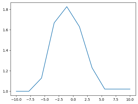
1D

meta.plot("proton/vg_rho")

[<matplotlib.lines.Line2D at 0x7fa125acb230>]

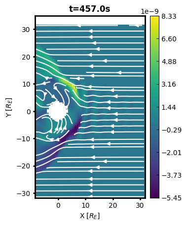
2D

file = "data/bulk.2d.vlsv"
meta = Vlsv(file)
meta.pcolormesh("vg_b_vol", comp=1)
meta.streamplot("proton/vg_v", comp="xy", color="w")

<matplotlib.streamplot.StreamplotSet at 0x7fa123756a50>

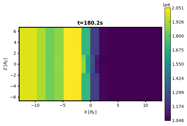
Field solver grid variables are also supported via the same APIs:

meta.pcolormesh("fg_b", comp=1)
meta.streamplot("fg_b", comp="xy", color="w")

<matplotlib.streamplot.StreamplotSet at 0x7fa1235a9d10>

2D slice of 3D AMR data

file = "data/bulk.amr.vlsv"
meta = Vlsv(file)
meta.pcolormesh("proton/vg_rho")

<matplotlib.collections.QuadMesh at 0x7fa12042f4d0>

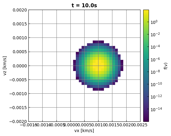
VDF

file = "data/bulk.1d.vlsv"
meta = Vlsv(file)
loc = [2.0, 0.0, 0.0]
meta.vdfslice(loc)

<matplotlib.collections.QuadMesh at 0x7fa1204d3610>