Wavelet Transform

There are already many nice introduction of wavelet transform, like here and the following video. This is my simple note on WT while reading those tutorials.

---

Before we talk about cross-wavelet transform (CWT), we need to first understand wavelet transform (WT). Conceptually wavelet transform is similar to Fourier transform, but with the main difference that wavelets are localized in both time and frequency whereas the standard Fourier transform is only localized in frequency . This means that for a given time series, Fourier analysis gives you precisely the frequency magnitude and phase across the whole time interval, but you cannot tell when in time the signal is sounded. Wavelet analysis takes the temporal extent into consideration by sacrificing the accuracy of the frequency spectrum.

The end result looks similar as if you perform a local Fourier tranform in a small time span around each time stamp (which is how the traditional spectrogram plots are done). The latter, which is also well-known, is called windowed Fourier tranform (WFT), where the FT is performed on short consecutive (overlapping or not) segments. The main limitation of this method is the lack of precision to either the time or the frequency domain. The size of the segment will determine either a high level of precision in the time domain or in the frequency domain. For example, a small window would not allow for the detection of any event larger than the window while maintaining a good localization in time. On the other end, a large window will take into account the long-term event (frequency domain) but with a high level of imprecision in the temporal domain.

Some more detailed explanation can be found in this Q&A.

Historically, the WT method was introduced in seismic research by Morlet (1983). Since then, wavelets are commonly used in geosciences as they are particularly well-suited in characterizing the “local” properties of time-series.

The joint characterization of the frequency content of the time-series in time while keeping a high level of precision in both time and frequency domains constitutes one of the WT advantages.

Time-Frequency Plane

FIGURE 1. Tiling of the time-frequency plane for the wavelet transform (WT) method. Narrow rectangles are used for the high frequencies that give a precise localization in time. Large rectangles are used for the low frequencies that give a precise localization in frequency. This illustrates the trade-off between the accuracy in time and the accuracy in frequency.

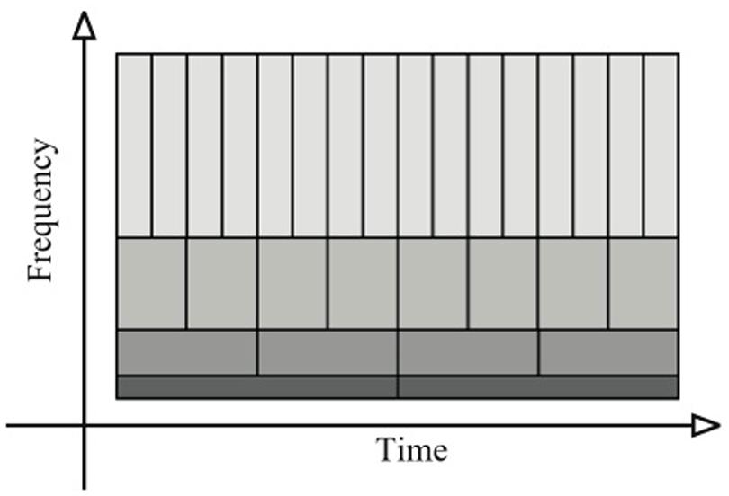
For the study of the WT, Flandrin (1988) called the time-frequency plane a scaleogram. In a scaleogram like Figure 1, we are able to perform a multi-scale analysis. One important line often shows up in a scaleogram is the cone of influence: within the region, the WT coefficient estimates are unreliable

Dilatation/Contraction/Translation of the Analyzing Function

A Wavelet is a wave-like oscillation that is localized in time. The WT is calculated by convolving the time-series s(t) with an analyzing wavelet function ψ(a,b) (derived from a mother function ψ) by dilatation of a and translation of b.¹

• a: scale factor that defines how “stretched” or “squished” a wavelet is. It determines the characteristic frequency so that varying a gives rise to a spectrum.
• b: translation in time, i.e. the “sliding window” of the wavelet over s(t). It determines where the wavelet is positioned in time. Location is important because unlike waves, wavelets are only non-zero in a short interval. Furthermore, when analyzing a signal we are not only interested in its oscillations, but where those oscillations take place.

Statistical Test

Intuitively, the WT coefficients near the edges of the time-series is less trust-worthy than in the middle. This observation can be captured analytically by performing a statistical test. Torrence and Compo, 1998 have demonstrated that, each point of the WT spectrum is statistically distributed as a chi-square with two degrees of freedom. The confidence level is computed as the product of the background spectrum (the power at each scale) by the desired significance level from the chi-square (\(\chi^2\)) distribution. When the WT spectrum is higher than the associated confidence level it is said to be “statistically significant.” Following this statistical test, we can obtain what is usually known as the cone of influence. See the MATLAB documentation for a live example.

In Production With Machine Learning

A nice post Multiple Time Series Classification by Using Continuous Wavelet Transformation introduces the idea of using continuous wavelet transform as a tool for data cleaning before feeding into convolutional neural networks. This is really a sweet spot where we can combine available math tools together to solve problems.

Tools

MATLAB

MATLAB has a mature wavelet toolbox.

Python

PyWavelets

Julia

The main package for wavelet in Julia is Wavelets.jl. Note that as of version 0.9.3, this package only supports discrete wavelet tranform. As an extension, ContinuousWavelets.jl implements the continuous wavelet transform, with some examples of scaleograms as well. I’m contacting the authors to see if it’s possible to extend the package even further.

Footnotes

1. The original inventors of WT used jargons like “dilation/contraction/translation” to describe the processes. I prefer to call them scale and shift.