AMReX Particle Data
We provide support for reading and analyzing AMReX particle data.
Loading Data
To load AMReX particle data:
data = AMReXParticle("path/to/data_directory")This will parse the header and prepare for lazy loading of particle data.
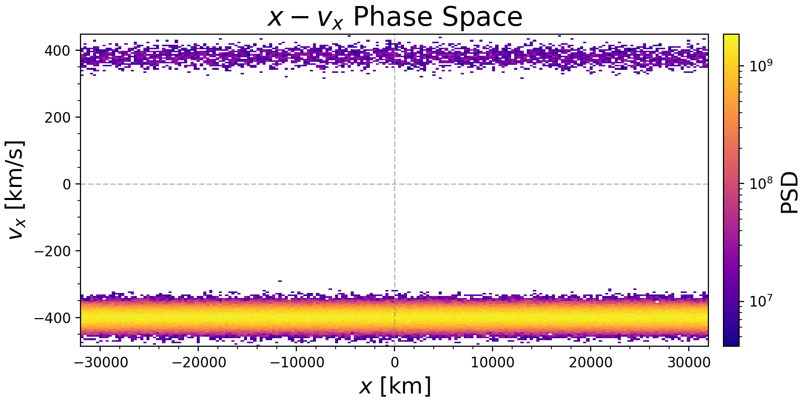
Phase Space Plotting
We can calculate and plot the phase space density distribution of particles.
First, load the PyPlot extension. The plot_phase function automatically calculates the density and plots it.
using PyPlot
plot_phase(data, "x", "vx";
bins=100,
x_range=(-10, 10),
y_range=(-5, 5),
log_scale=true,
plot_zero_lines=true,
normalize=true
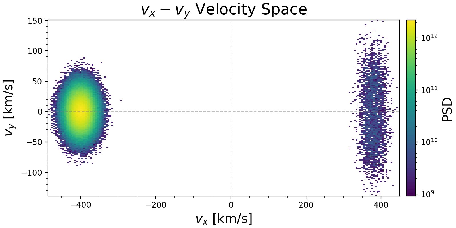
)Example plots for phase space ($x, v_x$) and velocity space ($v_x, v_y$) generated from AMReX particle data:
We can also calculate the phase space density histogram directly without plotting:
# 1D density
hist1d = get_phase_space_density(data, "vx")

# 2D density
hist2d = get_phase_space_density(data, "x", "vx"; bins=(100, 50))

# 3D density
hist3d = get_phase_space_density(data, "vx", "vy", "vz"; bins=50)

# Weighted 2D density (automatically detects "weight" component if present)
# or passes weights explicitly if not in data
hist2d_w = get_phase_space_density(data, "v_parallel", "v_perp")
We can also apply coordinate transformations to the particle data.
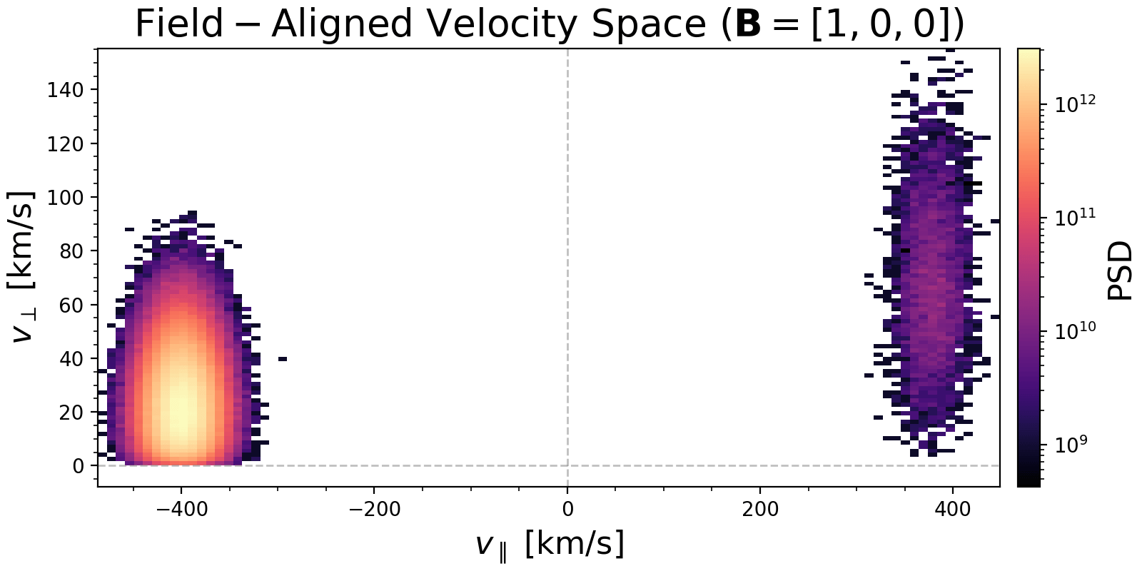
- Transformation with only B field. This decomposes velocity into parallel and perpendicular components relative to B.
transform_b = get_particle_field_aligned_transform([1.0, 0.0, 0.0])

plot_phase(data, "v_parallel", "v_perp";
   transform=transform_b,
   bins=50,
   log_scale=true
)
Example plot in field-aligned coordinates:
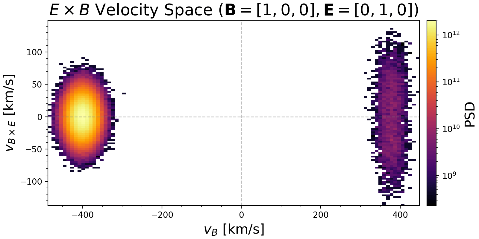
- Transformation with both B and E fields. This creates an orthonormal basis ($v_B$, $v_E$, $v_{B \times E}$), where $v_B$ is along B, $v_E$ is along the perpendicular component of E, and $v_{B \times E}$ is along the ExB drift direction.
transform_eb = get_particle_field_aligned_transform([1.0, 0.0, 0.0], [0.0, 1.0, 0.0])

plot_phase(data, "v_B", "v_BxE";
   transform=transform_eb,
   bins=50,
   log_scale=true
)
Example plot in ExB drift coordinates:
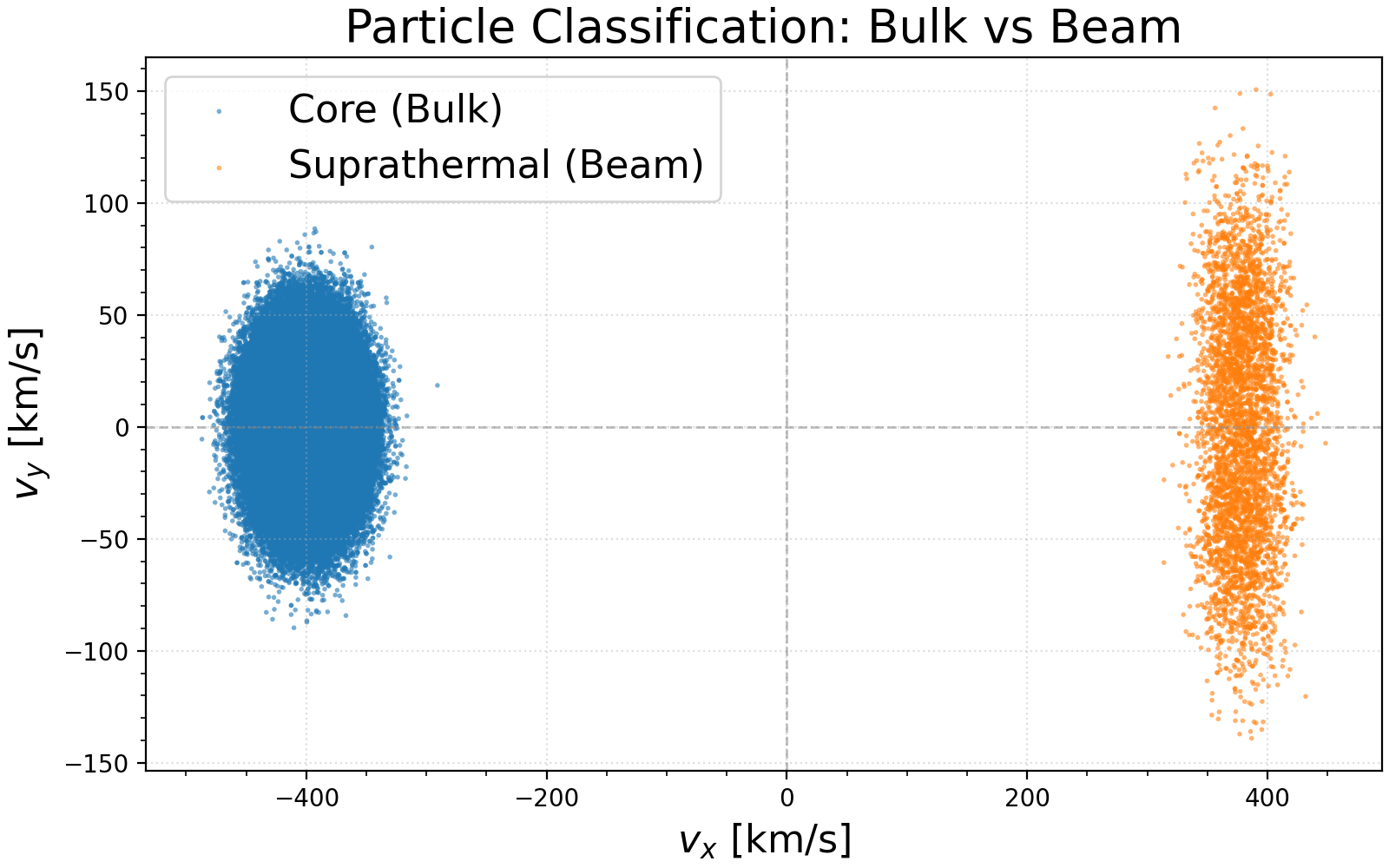
Particle Classification
You can classify particles into Core Maxwellian and Suprathermal populations using classify_particles. This function allows for specifying a spatial region and handling velocity distributions in 1D, 2D, or 3D.
# range can be specified by keywords x_range, y_range, z_range locally
core, halo = classify_particles(data;
    x_range=(-10000.0, 10000.0),
    y_range=(-30.0, 30.0),
    vdim=3,          # Velocity dimension (1, 2, or 3)
    vth=50.0,        # Core thermal velocity (required)
    nsigma=4.0,      # Separation threshold
    bulk_vel=nothing # Auto-detect if nothing
)
The function returns two matrices containing the classified particles. If bulk_vel is not provided, it is automatically estimated from the peak of the velocity distribution.
Visualizing Classification Results
You can visualize the core and suprathermal populations separately using PyPlot:
using PyPlot

# ... after classification ...

# Indices for velocity (e.g., "velocity_x", "velocity_y")
names = data.header.real_component_names
vx_idx = findfirst(==("velocity_x"), names)
vy_idx = findfirst(==("velocity_y"), names)

fig, ax = plt.subplots(figsize = (8, 5), constrained_layout = true)

# Scatter plot of Core and Halo
ax.scatter(core[vx_idx, :], core[vy_idx, :], s=4, label="Core (Bulk)", alpha=0.6)
ax.scatter(halo[vx_idx, :], halo[vy_idx, :], s=4, label="Suprathermal (Beam)", alpha=0.6)

ax.set_title("Particle Classification: Bulk vs Beam")
ax.set_xlabel(L"v_x \mathrm{~[km/s]}")
ax.set_ylabel(L"v_y \mathrm{~[km/s]}")
ax.axhline(0, color="gray", linestyle="--", linewidth=1, alpha=0.5)
ax.axvline(0, color="gray", linestyle="--", linewidth=1, alpha=0.5)

ax.legend()
ax.grid(true, linestyle=":", alpha=0.4)